Massachusetts Institute of Technology
Joint Program on the Science and Policy of Global Change

Report #37. Quantifying the Uncertainty in Climate Predictions

July 1998

Abstract

Uncertainties in projections of future climate change caused by an increase in greenhouse gas concentrations have been a subject of intensive study in recent years. However, in most cases, uncertainties in parameters and characteristics of models used to obtain those projections, such as climate sensitivity or radiative forcing, are described only by ranges of possible values. The resulting uncertainties in variables describing climate change, such as surface warming or sea level rise, are therefore also given just by ranges of possible values. However, for assessing the possible impact of climate change, it would be more useful to have probability distributions for these variables. There are two significant difficulties in obtaining such distributions. First, it is necessary to know probability distributions for the above mentioned uncertain parameters and model characteristics. Second, existing climate and economics models are computationally too expensive for traditional methods of uncertainty propagation such as Monte Carlo simulation.

We demonstrate a method for calculating probability distributions for surface air temperature change and sea level rise that result from uncertainties in climate sensitivity and the rate of heat uptake by the deep ocean. These distributions are obtained by applying the Deterministic Equivalent Modeling Method to the MIT climate model. This method provides an effective way of deriving an approximation for the model and allows the propagation of uncertainty. The range and probability distribution of climate sensitivity are based on expert assessments of parameters, while those for the rate of heat uptake are based on the results of simulations with coupled atmosphere-ocean GCMs. As an example of propagating correlated uncertainties, we also show the results of calculations in which the uncertainty in projected increases in forcing is also taken into account. The probability distribution for forcing, associated with an increase in atmospheric CO₂ concentrations is calculated based on the distributions for anthropogenic CO₂ emissions and the rate of oceanic carbon uptake. The probability distribution for emissions has been calculated in an independent study, while the rate of ocean carbon uptake is assumed to be related to that of heat.

Despite several decades of study, the climatic impacts of increasing greenhouse gases are still quite uncertain. The most detailed models, atmosphere-ocean general circulation models (AOGCMs), differ in the predicted climate change for a given increase in greenhouse gases. This uncertainty is further confounded by uncertainty in the future rate of increase of greenhouse gases. The large differences in future climate change predicted by current models, together with the need to address the risks of climate change through policy action, necessitate the evaluation of the uncertainty in projections of future climate change. Since we cannot give an exact prediction of climate, we would like to have estimates of the full range of possible outcomes and their relative likelihoods.

In any modeling endeavor, there are two distinct types of uncertainty: parametric uncertainty and structural uncertainty. Parametric uncertainty consists of uncertainty in values that a model's parameters should take. Structural uncertainty concerns uncertainty in the structure of a model, and is more difficult to treat in a rigorous and consistent fashion. For example, the differences in the responses of different AOGCMs to a given forcing are, to a large extent, due to differences in parameterizations of a variety of processes in the atmosphere-ocean-biosphere system, some of which are not yet well understood (Cess et al., 1990; Senior and Mitchell, 1993; Washington and Meehl, 1993). Another important uncertainty that accounts for different results from transient AOGCM simulations is the rate of heat uptake by the deep ocean (Murphy and Mitchell, 1995; IPCC, 1996). Models used in uncertainty studies usually include parameters allowing variation in model characteristics, such as climate sensitivity (Wigley and Raper, 1993, Murphy, 1995; DeWolde et al., 1997; Sokolov and Stone, 1998). This feature enables structural uncertainties to be treated as parametric ones. In this paper, we focus exclusively on the exploration of parametric uncertainty analysis, applied to parameters that represent structural uncertainties of AOGCMs.

There are different approaches to analyzing uncertainty in the parameters of a model. The method applied most frequently to climate models is sensitivity analysis. The sensitivity of a model to a parameter is defined to be the partial derivative of the model with respect to that parameter. Methods that compute these partial derivatives include the adjoint method, which enables the calculation of the sensitivity to all model parameters without rerunning the model (Hall, 1986; Hall and Cacuci, 1983). More commonly, sensitivity is explored through large discrete changes in a parameter value, by repeating a numerical simulation with the parameter in question set to a nominal, a low, and a high value, and all other parameters fixed. The change in the model's response(s) gives the model's sensitivity to that parameter. Multiple parameters may also be perturbed to high or low values at the same time to obtain an extreme value of a model response.

Most studies of uncertainty in climate models to date have been restricted to sensitivity analysis. The Second Assessment Report of the IPCC uses the sensitivity analysis approach to characterize the uncertainty in future climate change (IPCC, 1996). Simulations are performed on an energy balance-upwelling diffusion model of climate, varying the increase in future greenhouse gases over 6 different scenarios (IS92a-f), varying the climate sensitivity across the values 1.5^oC, 2.5^oC, and 4.5^oC, and varying the assumption about aerosols. Climate sensitivity is defined as the equilibrium change in globally averaged annual mean surface air temperature due to a doubling of the concentration of CO₂ in the atmosphere. A similar study is performed by Wigley and Raper (1993), who also examined uncertainty in the rate of heat uptake by the deep ocean, the depth of the ocean mixed layer, and the ratio of the temperature of polar-sinking water to the global mean temperature. Another set of sensitivity studies was performed with the MIT Integrated Global Systems Model (Prinn et al., 1998), examining the effects of uncertainty in greenhouse gas emissions, climate sensitivity, and heat and carbon uptake by the deep ocean.

One main disadvantage of sensitivity analyses is the inability to attach any measure of probability to the range of model responses. A class of methods that addresses these shortcomings includes methods of propagating probability distributions of parameters into probability distributions of outcomes, the best known of which is Monte Carlo. Monte Carlo simulations with a sample size of 4 runs have been performed by both Cubasch et al. (1994) and by Keen and Murphy (1997) to investigate the mean and variance of the transient response of an AOGCM with uncertainty in initial conditions. In general, however, a large number of simulations are required by the Monte Carlo approach to obtain reasonable approximations of probability distributions. Monte Carlo analysis is therefore usually too computationally expensive to be practical, and this partly accounts for the heavy reliance on sensitivity analysis in uncertainty studies. This paper uses a new method that makes uncertainty propagation feasible on computationally expensive models. The Deterministic Equivalent Modeling Method (DEMM) (Tatang et al., 1997) uses a small number of model runs to construct an approximation of the probabilistic response of the model.

In this paper DEMM is applied to the MIT 2D climate model (Sokolov and Stone, 1998) to derive probability distributions for global mean surface temperature change and sea level rise due to thermal expansion of the deep ocean. These distributions result from uncertainty in climate sensitivity, the rate of heat uptake by the deep ocean, and the rate of future increase in CO₂ concentrations.

Section 2 will describe the basic features of the MIT 2D climate model and our treatment of uncertainties. The impacts of uncertainty in climate sensitivity and the rate of heat uptake by the deep ocean on temperature change and sea level rise are explored in Section 3. In Section 4, the uncertainty in forcing due to increasing CO₂ will be included as a third source of uncertainty affecting temperature change and sea level rise. Section 5 will give conclusions.

2. DESCRIPTION OF THE MIT 2D CLIMATE MODEL: Transforming Structural Uncertainties into Parametric Uncertainties

The atmospheric component of the MIT 2D climate model (Sokolov and Stone 1998) is a modification of the GISS 2D dynamical-statistical model (Yao and Stone, 1987; Stone and Yao, 1987 and 1990) developed from the GISS GCM (Hansen et al., 1983). As a result, the model includes parameterizations of all the main physical processes and therefore is capable of reproducing many of the non-linear interactions simulated by atmospheric GCMs. At the same time, it is much more computationally efficient than existing GCMs. In simulations of present-day climate and equilibrium climate changes, the atmospheric model is coupled to a mixed-layer ocean model. The horizontal heat transport by the ocean is calculated from the results of a climate simulation with the MIT 2D model using climatological sea surface temperature and sea-ice distributions, and is held fixed in the climate experiments. In simulations of transient climate change the heat uptake by the deep ocean is parameterized by diffusive mixing of the mixed layer temperature's deviation from its present-day values (Hansen et al., 1984). Zonally averaged values of diffusion coefficients calculated from measurements of the tritium dispersal in the ocean are hereafter referred to as the "standard" values. These values for the diffusion coefficients vary from about 0.5 cm²/s in the equatorial region to about 5 cm²/s in high latitudes with a global average, denoted as K_v, equal to 2.5 cm²/s. Since in our model vertical diffusion is used to represent all processes responsible for heat penetration into the deep ocean, these values represent "effective" diffusion coefficients which are significantly larger than those used to represent subgrid scale mixing in oceanic GCMs.

One of the major uncertainties in climate modeling is the "climate sensitivity," which is defined as the increase in global mean temperature at equilibrium after a doubling of the atmospheric CO₂ concentration. While there are significant differences in climate sensitivity between different AGCMs, the climate sensitivity of any given AGCM is a fixed characteristic defined by the model's structure, such as its horizontal and vertical resolution, its parameterization of physical processes, etc. Thus, the climate sensitivity of the MIT 2D climate model is 3^oC. However, to study uncertainty in climate change one needs a model with "changeable" climate sensitivity. The versions of the MIT model with different climate sensitivities were obtained by inserting an additional cloud feedback; additional cloud feedback will result in greater warming at equilibrium from a CO₂ doubling, while less cloud feedback will reduce the eventual temperature. Specifically, the calculated cloud amount is multiplied by the factor (1 + kT_s), where T_s is the increase of the globally averaged surface air temperature with respect to its value in the present-day climate simulation (Hansen et al., 1993). Thus, different climate sensitivities can be obtained by an appropriate choice of the parameter k. As a result, the uncertainty in climate sensitivity can be treated as a parametric uncertainty. In the remainder of this paper, we refer only to the climate sensitivity directly, although simulations are in fact performed by setting a corresponding value for k.

As shown by Sokolov and Stone (1998), changes in different climate variables produced by different versions of the MIT 2D model are consistent with the results of GCMs with different climate sensitivities. It was also shown that the transient behavior of different AOGCMs can be matched by choosing appropriate values for climate sensitivity and for the rate of heat uptake by the deep ocean. The 2D climate model reproduces quite well both the increase of surface air temperature and the sea level rise due to the thermal expansion of the ocean as simulated by different AOGCMs for time periods of 100-150 years (Sokolov and Stone, 1998). The rate of heat uptake is adjusted by multiplying the "standard" diffusion coefficients by a constant factor at all latitudes, thereby preserving latitudinal structure. Such an approach allows one to change the rate of heat uptake by changing just one parameter, K_v. This again enables the structural uncertainty in the rate of heat uptake to be treated as a parametric uncertainty.

In general, the ability of the MIT 2D model to simulate the behavior of different AOGCMs makes it a useful tool for studying uncertainties in climate change projections.

3. UNCERTAINTY IN CLIMATE CHANGE FOR PRESCRIBED RADIATIVE FORCING

As discussed above, traditional Monte Carlo approaches to uncertainty propagation are not feasible for most climate models, even for simplified models such as the MIT 2D model. A recently developed methodology, the Deterministic Equivalent Modeling Method (DEMM) (Tatang et al., 1997; Webster, 1997), provides a feasible means of performing an uncertainty analysis on computationally expensive models. DEMM finds an optimal approximation of the response of a model with a minimal number of runs of the model. These approximations are truncated expansions of orthogonal polynomials, which are derived from the probability distributions assumed for the uncertain inputs. Once an approximation of the model output is found to be reasonably accurate, Monte Carlo simulations can be performed on the approximation to derive an approximate probability density function for the uncertain output. This process is depicted in Figure 1.

Figure 1. Uncertainty Propagation Using DEMM

The procedure for using DEMM for an uncertainty analysis consists of six steps:

1. Choose probability distributions for uncertain parameters,
2. Use input distributions to get parameter value sets to use in true model,
3. Run the true model,
4. Fit an approximation using results from model runs,
5. Check the accuracy of the approximation
6. Perform Monte Carlo on the approximation to obtain a probability density function of the model responses.

3.1 Uncertain Input Distributions

The first step of the analysis is to choose the probability distribution for the uncertain inputs. Unfortunately, information on probability for parameters such as climate sensitivity cannot be derived empirically, and must therefore rely on expert judgment. In the case of climate sensitivity, an elicitation has been performed for 16 climate science experts by Morgan and Keith (1995). The fractiles assessed from each expert is shown in Table 1. There is no standard way of combining judgments about probability from different experts. For this study, we chose to take the median of each of the fractiles (0.05, 0.25, 0.5, 0.75, 0.95), and use the median fractile values to fit a distribution. The resulting distribution is a beta distribution with shape parameters = 2.85, = 14.0 scaled over the range 0.0 to 15.0. The distribution for climate sensitivity is shown in Figure 2, along with the IPCC low, best guess, and high estimates.

Table 1. Subjective Probability Assessments of Climate Sensitivity

Expert	DT2x:0.05	DT2x:0.25	DT2x:Median	DT2x:0.75	DT2x:0.95
1	1	1.5	1.8	2.5	3.5
2	0.2	1.2	2.8	6	7.5
3	-1.5	1	2	4.8	6
4	0.8	1.5	2	4.5	6
5	0.2	0.2	0.5	1	1.2
6	-1	1.5	2.5	4	6
7	1	2	3	3.5	6.5
8	1	2	2.2	3.5	6
9	1	1.5	2.2	4	6
10	1	2	2.5	3	4
11	1.5	2	3	4	5
12	1.5	2	2.2	3	5.2
13	0.8	1.2	2	2.5	3.5
14	2	2.5	2.8	4	5
15	0.5	1.5	2	3	4.8
16	1.5	2	2.8	3.5	4.8
Median	1.00	1.50	2.20	3.50	5.10
Source: Morgan and Keith (1995)

Figure 2. Probability Density Function of Climate Sensitivity

The subjective probability assessments of the rate of heat uptake by the deep ocean were provided by Peter Stone and Andrei Sokolov (pers. comm., 1997). The "standard" values of diffusion coefficients (K_v = 2.5 cm²/s) obtained from observation of tritium mixing into the deep ocean, as described above, were chosen to be the median of the probability distribution for the rate of heat uptake by the deep ocean. The values of diffusion coefficients needed to match the transient behavior of different AOGCMs range from K_v = 0 cm²/s for the NCAR AOGCM to K_v = 25 cm²/s for the MPI model (Sokolov and Stone, 1998). Since both of those values do not seem to be highly probable, K_v = 0.5 cm²/s and K_v = 12.5 cm²/s were chosen as 0.05 and 0.95 fractiles respectively. The probability density function for the coefficient of heat uptake K_v is given in terms of its square root in Figure 3. The square root is used because the depth of penetration of a temperature change into the deep ocean, which defines the model response time, is proportional to the square root of the diffusion coefficient (see, for example, Hansen et al., 1985). The probability density function is a beta distribution, with shape parameters = 2.72, = 12.2 over a range of 0.0 to 10.0. Figure 3 also gives the values of the coefficient for heat uptake that allow the MIT model to reproduce the behavior of several AOGCMs (Sokolov and Stone 1998).

Figure 3. Probability Density Function of Square Root of Rate of Heat Uptake into Deep Ocean

Estimates of uncertainty in the rate of oceanic heat uptake based on observations are not available. However, IPCC (1996) does give an uncertainty range for the oceanic carbon uptake averaged over 1980s (2.0 +/- 0.8 PgC/year). In the MIT model, heat and carbon uptake by the deep ocean are treated similarly: coefficients for vertical diffusion of carbon are assumed to be proportional to those for heat (see Section 4). The values of oceanic carbon uptake averaged for the last five years of simulations with an off-line version of the oceanic carbon model, forced by the observed changes in atmospheric CO₂ from 1865 to 1984, are 1.11, 1.94 and 3.3 PgC/year, for diffusion coefficients with K_v equal to 0.5, 2,5 and 12.5 cm²/s, respectively. For K_v = 0.8 and K_v = 7.2 (+/- of the our distribution), the corresponding values of carbon uptake are 1.30 and 2.65 PgC/year. The ocean carbon uptake obtained in the simulation with diffusion coefficients corresponding to the median value of the proposed probability distribution is very close to the middle of the IPCC range, and the IPCC range is matched by values of diffusion coefficients lying between and 2. Thus, the assumed distribution for the rate of carbon uptake is consistent with the IPCC estimate of uncertainty in oceanic carbon uptake.

3.2 Accuracy of Collocation Approximation

Application of DEMM yields a third-order approximation including cross-terms that gives a very reasonable fit for decadal average temperature change and sea level rise. The approximation was derived from the results of 10 runs of the MIT 2D climate model, and evaluated by comparing results from 22 other runs at different parameter values. Figure 4 shows the accuracy in the approximations of temperature change and sea level rise in the last decade of a 100-year simulation. Note that a perfect approximation would always fall on the diagonal line.

Quantitatively, the average sum of squared errors of temperature change in the last decade is 0.77% of the mean. The error in the corresponding approximation for sea level rise in the last decade is 0.09% relative to the mean (Figure 4). In the DEMM approach, values of input parameters used for model runs are chosen to maximize the accuracy of the approximation in the high probability region of the parameter space. Because of the method of selecting parameter values, the accuracy of the obtained approximations is higher for more probable values of sensitivity and oceanic uptake. By the same token, some approximations may exhibit rather significant errors for parameter values close to the extremes of the chosen ranges. For example, the obtained approximations give negative values for sea level rise and negative temperature change for very low climate sensitivity and fast heat uptake.

Figure 4. Accuracy of Approximation of Temperature Change and Sea Level Rise in Last Decade

3.3 Resulting Uncertainty in Temperature and Sea Level Change

Using DEMM, we fit approximations for the decadal average surface temperature change and sea level rise for the last decade of a 100 year simulation. Figure 5 shows the derived probability distribution for average temperature change in the decade for years 91-100 of the simulations. These distributions result from 10,000 Monte Carlo simulations of the approximation, drawing from the input distributions in Figures 2 and 3.

Figure 5. Probability Density Function of Temperature Change in Last Decade of 100 Year Simulation

The temperature change in the last decade has a mean of 2.59^oC with a standard deviation of 1.09^oC. The probability density appears to be roughly Gaussian in shape. Figure 5 also shows that under these assumptions, there is still non-zero probability that the average decadal temperature rise exceeds 5^oC in the last decade. The probability density of average sea level rise in the same decade (Figure 6) also has an almost symmetric shape, with a mean of 15 cm and a standard deviation of 7 cm. Non-zero probabilities of zero increase of sea level and temperature are due to the above-mentioned errors of approximation at the extremes of the parameter distributions.

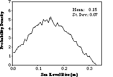
Figure 6. Probability Density Function of Sea Level Rise in Last Decade of 100 Year Simulation

Sensitivity analyses (such as IPCC, 1992, 1996; Prinn et al., 1998) give ranges of projections for surface warming and sea level rise as low, best, and high estimates. However, in reporting these and other uncertainty ranges, corresponding information about probabilities is usually not provided. For example, there is no indication whether the (low, high) range should be taken as a one standard deviation (67% confidence) interval, or a two standard deviation (95% confidence) interval, or an interval with some other level of confidence. In contrast distributions like those shown in Figures 5 and 6 give far more information than simple ranges. Thus, we can say that, under current assumptions about uncertainty in input parameters and for the assumed change in radiative forcing, an increase in annual mean global averaged surface temperature in 100 years with probability 67% will lie between 1.5 and 3.7^oC. Another important piece of information to decision-makers is the probability of damaging impacts that we wish to avoid. For example, the probability in this experiment that global mean surface temperature change after 100 years exceeds a value of 3.5^oC is 19.0%. Similar estimates can be obtained for any given value of surface warming or sea level rise.

Additional information can be obtained by examining the contours of surface temperature change and sea level rise as climate sensitivity and the rate of heat uptake range over their most likely values (K_v = 25 and T_eq = 5.1 are 0.95 fractiles of their distributions). Figures 7 and 8 illustrate the contours for temperature increase and sea level rise in the last decade. Contours for joint probability of input parameters are also shown in these figures by dashed curves, where the contour values indicate the probability of the input parameter taking on values in the area inside the corresponding contour. There is a clear difference in the dependence of temperature increase and sea level rise on the rate of heat uptake. While increase in temperature is a maximum for high sensitivity and low rate of heat uptake, sea level rise is a maximum for high sensitivity and high rate of heat uptake. It also can be seen from Figure 7, that the higher climate sensitivity, the stronger is the impact of heat uptake on surface warming. There is practically no such dependence for climate sensitivity less than 1.0^oC. The effect of increasing sensitivity on both surface temperature increase and the sea level rise, in turn, depends on the rate of heat uptake.

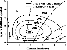
Figure 7. Contours of Temperature Change in Last Decade as a Function of Climate Sensitivity and Rate of Heat Uptake by Deep Ocean

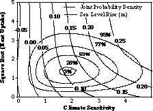
Figure 8. Contours of Sea Level Rise in Last Decade

3.4 Sensitivity to Assumptions about Uncertainty in Parameters

In the calculations above, the probability distributions of surface temperature increase and sea level rise are obtained for ranges of uncertainty in climate sensitivity and the rate of heat uptake by the deep ocean. However, it is not even known how to quantify these uncertainties. Because there is not sufficient observational evidence to constrain the uncertainty, we rely on the subjective beliefs of experts. As can be seen from Table 1, median values of climate sensitivity, as given by different experts, range from 0.5 to 3^oC. The given estimates of variance in climate sensitivity (i.e., the width of the probability distribution) are also rather different. Yet studies of expert assessment of uncertainties consistently show overconfidence (error bounds that are too small). Indeed, studies of several physical constants, such as the velocity of light or mass of an electron, show that (assuming current estimates to be "true" values) the error bars on previous estimated values almost never include the true value (Morgan and Henrion, 1990).

Here we test the sensitivity of output distributions to different assumptions about uncertainties in input parameters. In order to test the sensitivity, alternative probability distributions for both climate sensitivity and for the rate of heat uptake have been constructed. Two alternative distributions for climate sensitivity (Figure 9) have mean values of 1.5^oC and 3.0^oC and standard deviations of 0.4^oC and 1.2^oC, respectively. The median values for the alternative distributions of the rate of heat diffusion (Figure 10) correspond to K_v = 5 cm²/s and K_v = 1.25 cm²/s. As shown by Sokolov and Stone (1998), the first of those values matches the rate of heat uptake produced by the upwelling/diffusion model used by IPCC (1996), while the second one is chosen arbitrarily. Both of these values are well within the range of diffusion coefficients implied by the rates of heat uptake produced by different AOGCMs (Sokolov and Stone, 1998).

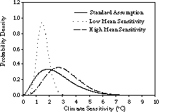
Figure 9. Alternative Probability Density Functions of Climate Sensitivity

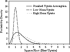
Figure 10. Alternative Probability Density Functions of the Rate of Heat Uptake into Deep Ocean

These probability distributions for climate sensitivity and the rate of heat uptake can be combined in different ways. All these combinations will lead to different resulting distributions for surface warming and sea level rise. Below we present the results for all four pairings of alternative input distributions. In order to obtain the most dramatic changes in the resulting distribution for surface temperature increase, we combined distributions with high mean climate sensitivity and slow mean heat uptake, hereafter referred to as the HS assumption, and the distributions with low mean sensitivity and fast mean uptake (LF assumption). The probability distributions for surface temperature increase and sea level rise obtained from these distribution pairs are shown in Figure 11 together with the distributions obtained under the "standard" assumptions (the results from Section 3.3). An increase/decrease in sensitivity tends to compensate a decrease/increase in the rate of heat uptake as far as sea level rise is concerned. Therefore, greater differences in sea level rise can instead be obtained by pairing high mean sensitivity with fast mean uptake (HF assumption) and low mean sensitivity with slow uptake (LS assumption). Figure 12 shows the distributions for surface temperature change and sea level rise for these two combinations of input parameters distributions. Various statistics of the resulting distributions obtained from alternative input distributions are summarized in Tables 2 and 3.

Figure 11. Probability Density Functions of Temperature Change and Sea Level Rise in Last Decade for Different Input Assumptions (HS and LF)

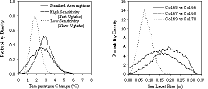
Figure 12. Probability Density Functions of Temperature Change and Sea Level Rise in Last Decade for Different Input Assumptions (HF and LS)

Table 2. Effects on Surface Temperature Change of Alternative Input Distributions

Assumption on input parameters	Mean	Standard Deviation	67% (+/- 1 s) Interval	Pr{T<1.0o}	Pr{T>3.0o}	Pr{T>3.5o}
Standard	2.59	1.09	(1.5, 3.7)	6%	36%	19%
LF assumptions	1.77	0.45	(1.3, 2.2)	3%	1%	0.1%
HS assumptions	3.31	1.00	(2.2, 4.2)	1%	62%	43%
HF assumptions	2.93	0.87	(2.0, 3.7)	1%	43%	23%
LS assumptions	1.88	0.51	(1.3, 2.3)	3%	2%	0.1%

Table 3. Effects on Sea Level Rise of Alternative Input Distributions

Assumption on input parameters	Mean	Standard Deviation	67% (+/- 1 s) Interval
Standard	0.15	0.07	(0.07, 0.23)
LF assumptions	0.10	0.04	(0.06, 0.14)
HS assumptions	0.16	0.55	(0.10, 0.21)
HF assumptions	0.19	0.65	(0.12, 0.26)
LS assumptions	0.08	0.03	(0.05, 0.11)

The resulting probability distributions for surface temperature change and sea level rise depend nonlinearly on the assumptions about the input parameter distributions. Thus, the mean value of temperature change for our "standard" distributions is significantly larger than for the LF combination. However, the probability of surface warming being less than 1^oC under our "standard" assumptions is twice as large as under both LS and LF distribution pairings. This is caused by the fact that the low mean climate sensitivity distribution has much lower variance than the standard distribution for climate sensitivity. This smaller variance, together with the weak dependence of surface temperature increase on the rate of heat uptake for low climate sensitivity, results in a rather narrow 67% probability range of surface warming for the LS and LF combinations.

The probability of surface temperature rising by more than 3^oC, while mainly determined by the assumed distribution for climate sensitivity, is also sensitive to the distribution for the rate of oceanic heat uptake. As mentioned above, the dependence of the projected change in surface temperature on the rate of oceanic heat uptake rapidly increases with an increase in climate sensitivity. Because of that, the difference between the upper bounds of the 67% probability intervals under the HS and HF cases are much larger than the difference between the corresponding lower bounds. Both the mean value and the width of the 67% probability interval of the resulting distributions for sea level rise are also noticeably different for different assumptions regarding input parameters.

As can be seen from the above results, the resulting probability distributions for the climate variables in question differ significantly depending on the assumed probability distributions of climate sensitivity and the rate of oceanic uptake. Therefore, it would be useful to be able to constrain the possible values of these parameters of the climate system. A study aimed to obtain such constraints using fingerprint detection techniques is currently ongoing within the MIT Joint Program on the Science and Policy of Global Change (Forest, Allen and Sokolov, 1997).

4. UNCERTAINTY IN CLIMATE CHANGE WITH UNCERTAINTY IN CARBON EMISSIONS

Probability distributions of temperature change and sea level rise shown in the previous section are associated with uncertainties in climate sensitivity and the rate of heat uptake by the deep ocean. However, there is also a significant uncertainty in future radiative forcing. The latter uncertainty, in turn, arises from uncertainties in greenhouse gas emissions, radiative effects of aerosols, and so on. The MIT Integrated Global System Model (IGSM), which includes interactive climate chemistry model (Wang et al., 1998), oceanic carbon model (Prinn et al., 1998) and Emissions Prediction and Policy Analysis (EPPA) model (Yang et al., 1996; Jacoby et al., 1997), can be used for studying most of the above uncertainties. Results of a sensitivity study performed with the IGSM, in which most of the above uncertainties are considered, are described in Prinn et al (1998). However, the IGSM is too computationally expensive to be used directly in a Monte Carlo type uncertainty study. Below we present the results of Monte Carlo simulations performed as in the previous section. These results, along with the uncertainty in climate sensitivity and heat uptake by the deep ocean, take into account uncertainty in forcing associated with uncertainty in CO₂ emissions.

4.1 Propagating Emissions Uncertainty from an Economic Model

There are two sources of uncertainties in future CO₂ emissions, namely uncertainties in parameters and structure of economic models and uncertainty in future policies. Uncertainty in CO₂ emissions, resulting from uncertainties in three parameters of the EPPA model, for a reference or no-policy case has been studied by Webster (1997) using the DEMM approach. As a result of this study, projected CO₂ emissions for the years 1990-2100 were parameterized by third order polynomials of these parameters, with coefficients that depend on time. Similar approximations can be found for any policy; but for the first experiments with the climate model we are mainly interested in developing way for propagating the economic uncertainty and therefore restrict ourselves to the reference or no-policy case

A straightforward approach for estimating uncertainty in projected climate change resulting from uncertainties in CO₂ emissions, climate sensitivity and the rate of oceanic heat and carbon uptake would be to perform simulations similar to those described in the previous section with the full IGSM. This approach is not efficient for two reasons. First it would require fitting the IGSM with a polynomial of five variables (three economic and two climate parameters), while in fact the climate-chemistry model only treats emissions as a single input conceptually. In using DEMM to produce an approximation of a more complex model, the number of input parameters and the order of the polynomial fit are the determinants of the number of runs required of the original model, and thus of the computational expense. Since in the IGSM, the coefficient for vertical diffusion of carbon is assumed to be proportional to that for heat (Prinn et al., 1998), there is no additional uncertainty associated with the rate of the oceanic carbon uptake. Second, the climate-chemistry model needed to calculate CO₂ concentration from emissions is about three times more expensive computationally than just the climate model used in the previous section.

The results of previously performed simulations with the climate-chemistry model have shown that CO₂ concentration is mainly defined by the CO₂ emissions and the rate of oceanic carbon uptake and is not sensitive to predicted changes in atmospheric temperature and humidity, and thus to climate sensitivity (Prinn et al., 1998). Therefore, if increases in atmospheric CO₂ concentration can be described by a unique function of the whole range of possible emissions and rates of carbon uptake, then the necessary simulations can be performed with just the climate model, forced by the prescribed changes in atmospheric CO₂, and the computational cost of creating DEMM approximations will be greatly reduced. If this function depends on less than three (number of uncertain parameters in EPPA model) parameters it will also decrease the total number of input parameters and, as a result, decrease the number of runs with the real model needed to obtain approximations.

Possible paths of CO₂ concentrations were calculated using the above approximation of the EPPA model and an oceanic carbon model. Initial distributions of the carbon in the ocean for different values of vertical diffusion coefficients were obtained by means of off-line runs with the ocean carbon model. In those runs, the model was forced by a CO₂ concentration changing according to observations from 1765 to 1985, starting from equilibrium. Projections of CO₂ concentrations for three sets of parameters are shown in Figure 13. Values of economic parameters and the rate of oceanic carbon uptake in those runs correspond to high, reference and low cases of the sensitivity study with the IGSM model described by Prinn et al. (1998).

In spite of significant differences in values of economic parameters used in these cases, CO₂ emissions produced by the EPPA model are almost identical up to the year 2000 (Prinn et al., 1998). In addition, projected CO₂ concentration is determined not by just oceanic carbon uptake, but also by the carbon uptake by the terrestrial ecosystem. While present-day values of both oceanic and terrestrial uptake are uncertain, the total carbon uptake is fairly well known from the data for carbon emissions and the increase in atmospheric CO₂ concentration for the recent past. Values of the terrestrial carbon uptake used in the simulations with different values of vertical diffusion coefficients were calculated as the difference between the prescribed total uptake (4.1 PgC/year) and the value of oceanic uptake averaged over the last five years of the off-line simulation. As a result, total carbon uptake is essentially the same during the initial stages of all simulations, regardless of the rate of oceanic uptake. Because of the similarity in emissions and the constraint on total carbon uptake, there is virtually no difference between projected CO₂ concentrations for different values of input parameters until the year 2010 (Fig. 12, see also Prinn et al., 1998, Fig. 28).

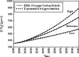
Figure 13. CO₂ Concentrations for Reference, High, and Low Cases and for Corresponding Percentage Increase Approximations

A variety of functional forms with one or two parameters were tested to see which could reproduce a variety of concentration paths over the whole range of economic parameters and the rate of carbon uptake. It was found that changes in atmospheric CO₂ concentrations for the years 2010-2100 can be very accurately approximated by a annually compounded percentage increase from an initial value. The values for concentration in 1985-2009 use the corresponding concentrations for the EPPA run with reference values for all uncertain parameters. Thus the procedure to find a single number to construct an equivalent concentration path for a given set of EPPA parameter values and rate of oceanic carbon uptake is:

1. Use emissions metamodel to find emission path over time for given set of economic parameters;
2. Use the oceanic carbon model to find the concentration path for the given emission path and the given rate of oceanic carbon uptake;
3. Find the percentage rate a which solves:

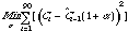where C_i is the concentration for year i and C_j is the approximation based on exponential growth at rate a.

A graphic demonstration of the accuracy yielded by this approach is given in Figure 13, which shows concentration profiles for reference, high emissions, and low emissions scenarios from EPPA and oceanic carbon model and the optimal percentage rate approximation for each of them. Note that the approximations are visually indistinguishable.

With this approach, the distributions for the three economic uncertainties and the rate of oceanic carbon uptake can be propagated through the emissions metamodel, oceanic carbon model, and optimal fit procedure to yield a distribution of CO₂ rates of increase that reflects those uncertainties. This distribution can then be used as a third uncertain input into the MIT 2D climate model.

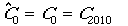
Using the above procedure as a "true" model, a third order polynomial approximation is used to create a metamodel that directly calculates a percentage rate of CO₂ increase as a function of the four uncertain inputs. Figure 14 shows the probability distributions for the four uncertain input parameters. Figure 15 demonstrates graphically the accuracy of this model on 39 runs of the actual fitting procedure. The sum of squared deviations is 0.01% of the mean. Performing 10,000 Monte Carlo simulations of this metamodel with sampling from the four input distributions (Figure 14) yields a derived probability distribution for the percentage rate of increase of CO₂, shown in Figure 16.

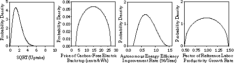
Figure 14. Probability Density Functions of Uncertain Parameters to Determine Forcing

Figure 15. Accuracy of Approximation of Rate of CO₂ Increase

Figure 16. Probability Density Function for Rate of CO₂ Increase Uncertain Uptake vs. Fixed Uptake

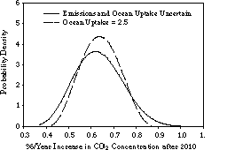
The IPCC presents alternative atmospheric CO₂ scenarios resulting from differences in carbon emissions, but uncertainty in the oceanic carbon uptake is not taken into account (IPCC, 1996). The approach described above allows us to estimate relative contributions of uncertainties in emissions and carbon uptake to the resulting uncertainty in projected CO₂ concentrations. Figure 16 compares the distribution where uptake is uncertain to the case where uptake is fixed at the reference value of 2.5 cm²/s. While the means of both distributions are similar (0.69%/year for all uncertainties versus 0.71%/year in the fixed uptake case), the variance is noticeably smaller when uncertainty in carbon uptake is ignored. Our calculation shows that under the assumed probability distributions for the input parameters, 38% of the uncertainty in the rate of CO₂ increase is associated with uncertainty in the rate of oceanic carbon uptake. This leads to a 28% increase in the range of uncertainty for radiative forcing in 2100; the 90% probability range for the radiative forcing due to the increase in CO₂ from 1990 to 2100 is 3.62-5.12 W/m² for the fixed diffusion case, and 3.38-5.42 W/m² if uncertainty in carbon uptake is included (Figure 17).

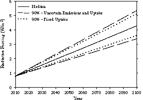
Figure 17. Radiative Forcing due to Increasing CO₂ Uncertain Uptake vs. Fixed Uptake

The median forcing in our simulations is somewhat smaller than that for IPCC scenario IS92a or for the reference case in Prinn et al. (1998). This is because in this study increases in greenhouse gases other than CO₂ are not taken into account. As a result, the range of uncertainty in forcing here is narrower than in Prinn et al. (1998). In addition to considering other greenhouse gases, IPCC (1996) also includes differences in future policies, and thus its uncertainty ranges are not directly comparable to the ranges given here.

The probability distribution in Figure 16 is in no way a definitive description of uncertainty in emissions, because it is based on only a few of many uncertainties and uses one of many possible parameterizations of economics and the carbon cycle. Nevertheless, the method by which it is obtained provides an analytical basis for choosing "central" and other scenarios. If there is such a distribution underlying the judgment of the likelihood of IS92a, it has not been presented.

4.2 Resulting Uncertainty in Temperature Change and Sea Level Rise due to Thermal Expansion

Using the distribution of the rate of CO₂ increase from Section 4.1, as well as the distributions for climate sensitivity and rate of heat uptake from Section 3.1, new third order approximations for model responses are obtained from 20 simulations of the MIT 2D climate model. In addition, 23 simulations were performed at parameter values equidistant in probability space between the values to fit the approximation. The accuracy of the approximations of temperature change and sea level rise in the last decade for these 23 100-year simulations is shown in Figure 18. Although the constructed approximation tends to underestimate sea level rise at higher values, the normalized sum of square deviations is less than 0.5% of the mean value. The corresponding value for the approximation of temperature increase is 1.3%.

Monte Carlo simulations were performed with these approximations of temperature change and sea level rise. However, there is one additional step required in the procedure. The uncertainty in heat uptake is not only an input into the climate model, but is also an uncertain input into the sink.

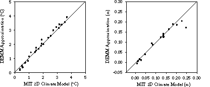
Figure 18. Accuracy of Approximations of Temperature Change and Sea Level Rise in Last Decade Including Uncertainty in Rate of CO₂ Increase

The uncertainty in CO₂ increase is therefore correlated with the uncertainty in heat uptake ^[1], and this correlation must be accounted for when propagating these uncertainties through the climate determination of the distribution of the rate of CO₂ increase in the model of the oceanic carbon model. The rate of heat uptake is assumed to be proportional to the rate of CO₂ uptake by the ocean, and so a higher value of uptake means less CO₂ in the atmosphere, thus a slower increase in concentrations.

A modified Monte Carlo procedure is used to sample from the three-parameter distributions and derive probability distributions for decadal average changes in surface temperature and sea level. When generating the parameter set for each Monte Carlo simulation, a value of heat uptake is first sampled from its distribution. The procedure then uses the Copula method (Clemen and Reilly, 1997) to derive a conditional distribution for CO₂ increase given that value of heat uptake. The conditional distribution is sampled to obtain a random but correlated value for CO₂ increase. The resulting probability density functions for surface temperature change and sea level rise in the last decade of 100-year simulations that result from uncertainty in climate sensitivity, heat uptake, and CO₂ emissions are given in Figures 19 and 20.

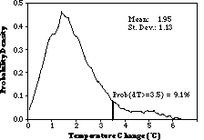
Figure 19. Probability Distribution of Temperature Change in Last Decade of 100 Year Simulation Including Uncertainty in Rate of CO₂ Increase

Figure 20. Probability Distribution of Sea Level Rise in Last Decade of 100 Year Simulation Due to Thermal Expansion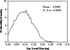

Uncertainties in the transient model response to the gradual increase in CO₂ concentration can be studied by obtaining similar approximations and probability distributions for each decade of simulations. Using these distributions, the 90% probability bounds are calculated for decadal average surface temperature change and sea level rise (Figures 21 and 22). Although these graphs may appear similar to several figures in the IPCC Second Assessment Report portraying projected global mean surface temperature changes and sea level rise, in the sense of having low, middle, and high projections, the information content is different. In particular, we think that graphs such as Figures 21 and 22 contain more information by displaying the amount of probability that the modeled "true" value of temperature change will be within the bounds given. Since assessments of the uncertainty in projected climate change are intended to inform policy decisions, which concern trading off risks of climate change against costs of mitigation, attaching probability to uncertainty bounds can increase the usefulness of such studies.

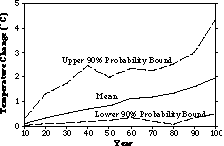
Figure 21. 90% Probability Interval for Decadal Average Global Mean Temperature Change

Figure 22. 90% Probability Interval for Decadal Average Sea Level Rise Due to Thermal Expansion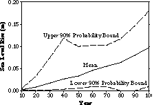

The results for transient changes in surface temperature and sea level shown above should be viewed with caution. Surface temperature, as well as any other climate variable predicted in climate change simulations, can be represented as a sum of two main components: a response to the imposed external forcing and an internal natural variability. The internal variability for any given climate model can be calculated from the results of a present-day equilibrium climate simulation run for many years. The standard deviation of an annual mean global average surface temperature for the MIT 2D climate model is 0.06^oC (Sokolov and Stone, 1998), which is half as large as the corresponding value for coupled AOGCMs. Depending on the values of model parameters, the effect of natural variability may overwhelm the model response resulting in a surface temperature change that is higher or lower than expected. The effect of natural variability is most noticeable in the early years of a transient simulation, especially when the forcing increases slowly. As discussed by Cubash et al. (1994) and by Kenn and Murphy (1997), the contaminating effect of natural variability can be reduced by carrying out an ensemble of climate change simulations from different initial conditions. The detection time for an increase in surface temperature, defined as the time at which the difference between projected surface temperature and its value in a control run exceeds two standard deviations, is about ten years less for an ensemble average than for individual integrations (Cubash et al., 1994; Kenn and Murphy, 1997). All results presented in this study are based on the results of the simulations carried out only from one set of initial conditions.

4.3 Relative Contribution to Uncertainty by Uncertain Parameters

The previous sections have shown how DEMM can be used to efficiently propagate uncertainty in parameters to obtain descriptions of the uncertainty in model responses. Because of the ease of propagating different uncertainties through the approximations, we can also examine the relative contribution to uncertainty in temperature change or sea level rise from individual or subsets of uncertain parameters.

As an example below we consider the relative role of economic uncertainties that determine emissions versus physical uncertainties about the climate system in affecting the uncertainty in climate impacts. The uncertainty in forcing due to CO₂ increase derived in Section 4.1 is a function of both the economic uncertainties and the uncertainty in ocean uptake of carbon. Alternative distributions for forcing can be derived using only economic uncertainties (with uptake fixed at the reference value) and again using only uncertainty in ocean uptake (using reference emissions). By using the distribution for forcing with only economic uncertainties, and fixing climate sensitivity and heat uptake also at reference values, the uncertainty in temperature change and sea level rise due only to emissions uncertainties is obtained. Similarly, the forcing distribution for uncertain uptake only is used along with the uncertainties in climate sensitivity and heat uptake to obtain the contribution of only the physical uncertainties.

The results for decadal average temperature change are shown in Figure 23 and for decadal average sea level rise in Figure 24, both for the last decade of a hundred-year simulation. In both cases, the physical uncertainties are driving the majority of the uncertainty in impacts. However, because neither the economic nor the physical uncertainties treated here include all the important sources of uncertainty, the ranges given are not definitive results. Nevertheless, these results illustrate the type of analysis that can be used to prioritize research focused on reducing uncertainty. Were the results of a more complete study to resemble the ones shown here, they would suggest that while economic processes are not insignificant, improving our understanding of the climate system should be a primary focus for research. Such an analysis should also consider which uncertainties are more likely to be resolved in considering priorities.

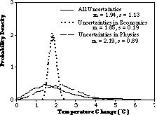
Figure 23. Probability Distribution of Temperature Change in Last Decade Relative Contribution of Economic Uncertainties vs. Physical Uncertainties

Figure 24. Probability Distribution of Sea Level Rise in Last Decade Relative Contribution of Economic Uncertainties vs. Physical Uncertainties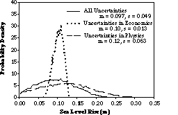

5. CONCLUSIONS AND FUTURE WORK

This paper has presented probability distributions for responses from a climate model that result from uncertainty in some key parameters. These distributions were obtained by applying the Deterministic Equivalent Modeling Method, which captures the major non-linear behavior of uncertain parameters in determining model responses.

The set of results presented is preliminary. The results focus only on uncertainty in forcing due to CO₂ emissions, neglecting uncertainty in emissions in aerosols and other trace gases. Other uncertainties such as the effect on radiative forcing of aerosols and uncertainty in initial conditions were also neglected in this study. Finally, the uncertainty in forcing from CO₂ does not include the contribution from all the important sources of economic uncertainty. Nevertheless, many important pieces of information can be obtained from an application of this method:

* An effective method for obtaining probability distributions for changes in climate variables based on the uncertainty in climate and economic input parameters.

* Probability distributions and 90% probability bounds on responses over time give more information than simple ranges, and may be more useful to policy discussions.

* Probability distributions and response contours help to give an understanding of how key parameters affect model responses.

* Relative contributions of uncertainties in different input parameters to resulting uncertainties in climate response.

Acknowledgments

We wish to thank Dick Eckaus, Jake Jacoby, Ron Prinn, Peter Stone, and Vince Webb for their help and support. The work presented here is a contribution to MIT's Joint Program on the Science and Policy of Global Change. The Joint Program is supported by a government-industry partnership that includes the U.S. Department of Energy (901214-HAR; DE-FG02-94ER61937; DE-FG02-93ER61713), U.S. National Science Foundation (9523616-ATM), U.S. National Oceanic and Atmospheric Administration (NA56GP0376), and U.S. Environmental Protection Agency (CR-820662-02), the Royal Norwegian Ministries of Petroleum and Energy and Foreign Affairs, and a group of corporate sponsors from the United States, Europe and Japan.

REFERENCES

Cess, R.D., et al. (1990). Intercomparison and interpretation of climate feedback processes in 19 atmospheric general circulation models, J. Geophysical Research, 95:16,601-16,615.

Clemen and Reilly, J. (1997). Correlations and copulas for decision and risk analysis, DRAFT, March, 1997.

Cubasch, U., et al. (1994). Monte Carlo climate change forecasts with a global coupled ocean-atmosphere model, Climate Dynamics, 10:1-19.

DeWolde, J. R., P. Huybrechts, J. Oerlemans and R.S.W. Van de Wal (1997). Projection of global mean sea level rise calculated with a two-dimensional energy-balance climate model and dynamic ice sheet models, Tellus, 49A, 486-502.

Forest C.E., M.R. Allen and A.P. Sokolov (1997). Constraining climate model parameters using climate observations, EOS Transactions, 78(46):128.

Hall, M.C.G. (1986). Application of adjoint sensitivity theory to an atmospheric general circulation model, J. Atmospheric Sciences, 43(22):2644-2652.

Hall, M.C.G. and D.G. Cacuci (1983). Physical interpretation of the adjoint functions for sensitivity analysis of atmospheric models, J. Atm. Sci., 40:2537-2546.

Hansen, J., et al. (1993). How Sensitive is the World's Climate?, National Geographic Research and Exploration. 9:142-158.

Hansen, J., et al. (1988). Global climate change as forecast by Goddard Institute for Space Studies three-dimensional model, J. Geophys. Res. 93:9341-9364.

Hansen, J., G. Russel, A. Lacis, I. Fung, D. Rind and P. Stone (1985). Climate response time: dependence on climate sensitivity and ocean mixing, Science, 229:857-859.

Hansen, J., et al. (1984). Climate sensitivity: Analysis of feedback mechanisms, in: "Climate Processes and Climate Sensitivity," Geophysical Monograph Series, 29, J. Hansen and T. Takahashi, eds., AGU, pp. 130-163.

Hansen, J., et al. (1983). Efficient three-dimensional global models for climate studies: Models I and II, Monthly Weather Review, 111:609-662.

IPCC (1996). Climate Change 1995 - The Science of Climate Change, Contribution of Working Group I to the Second Assessment Report of the Intergovernmental Panel on Climate Change, J.T. Houghton, L.G. Meira Filho, B.A. Callander, N. Harris, A. Kattenberg, and K. Maskell, eds., Cambridge U. Press: Cambridge, UK.

Jacoby, H.D., R.S. Eckaus, A.D. Ellerman, R.G. Prinn, D.M. Reiner and Z. Yang (1997). CO₂ emissions limits: Economic adjustments and distribution of burdens, Energy Journal, 18(3):31-58.

Keen, A.B., and J.M. Murphy (1997). Influence of natural variability and the cold start problem on the simulated transient response to increasing CO₂, Climate Dynamic, 13:847-864.

Morgan M.G., and M. Henrion (1990). Uncertainty: A Guide to Dealing with Uncertainty in Quantitative Risk and Policy Analysis, Cambridge University Press: New York.

Morgan, M.G., and D.W. Keith (1995). Subjective judgements by climate experts, Environmental Policy Analysis 29(10):468A-476A.

Murphy, J.M. (1995). Transient response of the Hadley Center coupled ocean-atmosphere model to increasing carbon dioxide. III: Analysis of global-mean responses using simple models, J. Climate, 8:496-514.

Prinn, R., et. al. (1998). Integrated global system model for climate policy analysis: Feedbacks and sensitivity studies, Climatic Change, in press (available as Report No. 36, JPSPGC, MIT, Cambridge, MA).

Senior, C.A., and J.F.B. Mitchell (1993). Carbon dioxide and climate: The impact of cloud parameterization, J. Climate, 6:393-418.

Sokolov, A.P. and P.H. Stone (1998). A flexible climate model for use in integrated assessments, Climate Dynamics, 14:291-303.

Stone, P.H., and M.-S. Yao (1987). Development of a two-dimensional zonally averaged statistical-dynamical model. II: The role of eddy momentum fluxes in the general circulation and their parameterization, J. Atm. Sci., 44:3769-3536.

Stone, P.H., and M.-S. Yao (1990). Development of a two-dimensional zonally averaged statistical-dynamical model. III: The parameterization of the eddy fluxes of heat and moisture, J. Climate, 3:726-740.

Tatang, M.A., W. Pan, R.G. Prinn and G.J. McRae (1997). An efficient method for parametric uncertainty analysis of numerical geophysical models, J. Geophys. Res., 102(D18):21,925-21,932.

Washington, W.M., and G.A. Meehl (1993). Greenhouse sensitivity experiments with penetrative cumulus convection and tropical cirrus albedo effects, Climate Dynamics, 8:211-223.

Wang C., R.G. Prinn, A.P. Sokolov (1998). A global interactive chemistry and climate model: Formulation and testing, J. Geophys. Res., 103(D3):3399-3418.

Webster, M.D. (1997). Exploring the uncertainty in future carbon emissions, Report No. 30, Joint Program on the Science and Policy of Global Change, MIT, Cambridge, MA, December.

Wigley, T.M.L. and S.C.B. Raper (1993). Future changes in global mean temperature and sea level, in: Climate and Sea Level Change: Observations, Projections, and Implications, R. Warrick, E. Barrow and T. Wigley, eds., Cambridge University Press: Cambridge, UK.

Yao, M.-S., and P.H. Stone (1987). Development of a two-dimensional zonally averaged statistical-dynamical model. I: The parameterization of moist convection and its role in the general circulation, J. Atmos. Sci., 44:65-82.

Yang, Z., R.S. Eckaus, A.D. Ellerman and H.D. Jacoby (1996). The MIT Emissions Prediction and Policy Analysis (EPPA) Model, Report No. 6, Joint Program on the Science and Policy of Global Change, MIT, Cambridge, MA.

| Top of page | | |