Massachusetts Institute of Technology
Joint Program on the Science and Policy of Global Change

Report #38. Sequential Climate Decisions Under Uncertainty: An Integrated Framework

September 1998

Abstract

In this paper, we present an integrated framework for structuring and evaluating sequential greenhouse gas abatement policies under uncertainty. The analysis integrates information concerning the magnitude, timing, and impacts of climate change with data on the likely effectiveness and cost of possible response options, using reduced-scale representations of the global climate system drawn from the MIT Integrated Global System Model. To illustrate the method, we explore emissions control policies of the form considered under the United Nations Framework Convention on Climate Change.

1. INTRODUCTION

International efforts to negotiate a response to the threat of climate change have spawned research on improved methods for characterizing this difficult issue, and for analyzing emissions control options. One focus of this work has been a class of applications commonly referred to as integrated assessment models, which seek to pull together the many features of the problem into a coherent, consistent framework.[1] As pointed out by the Intergovernmental Panel on Climate Change (IPCC), analysts working on the issue face two main challenges [3]:

* Integrating and managing a large and diverse array of data and models from many researchers and a range of disciplines;

* Improving the relevance of the models to policy needs, as well as the presentation of model results to policymakers.

The analytical approach explored here is a step towards satisfying these objectives. We present a policy-oriented, integrated decision analysis (IDA) framework that focuses specifically on the fact that decisions about greenhouse gas control are not made once and for all; current policy choices will be reconsidered in future years in light of new data and increased understanding about the problem. Few integrated assessments take explicit account of the sequential character of climate decisions, sometimes because of lack of familiarity with the range of analytic techniques that can be used to model these types of problems, but more often because the computational support for these methods has been primitive, and the calculations prohibitive in cost. Of course, policymakers know that decisions will be reconsidered over time,particularly for a long-run issue like climate change. If analysis cannot deal explicitly with this aspect, its value in informing climate policy decisions is diminished.

In developing our analytic framework, we build on previous applications of decision-oriented models in the climate area.[2] Two main features characterize our approach, and each is occasioned by the peculiar complexity and scope of the climate change issue. First, we represent uncertainty about the response of the climate system to human emissions in terms of key variables that are used by climate scientists as part of their modeling and analysis efforts. This formulation is a useful extension of previous efforts, most of which apply a single, highly-summarized indicator of "high" vs. "low" response, in terms of some climatic effect or overall social impact.[3] Stating uncertainty in terms of key physical variables that drive climate analysis models provides a more informative picture of uncertainty in the climate machine. It also facilitates communication with climate scientists, particularly in the crucial step of elicitating probabilistic expert judgements about these uncertain quantities and their likely resolution over time.

Second, we estimate key empirical relations using a single, integrated set of models of the global climate system. Because of its computational requirements,a sequential decision analysis must be based on relatively simple mathematical representations of underlying processes. In the analysis presented below, there are five such components: (i) the trajectory of greenhouse emissions; (ii) the effect of these emissions on atmospheric concentrations; (iii) the translation of concentrations to radiative forcing; (iv) the response of climate to this forcing; (v) the impacts of any change in climate; and (vi) the economic valuation of these changes. Models used by specialists in each of these domains are large and complex, and to integrate them into a framework useful for policy analysis they must be recast in simpler forms. We shall refer to a small,nimble version of the components of a large and complex model as a reduced-scale representation. Estimating reduced-scale model parameters from a single, more-detailed framework makes it possible to document the basis for the analysis. Also, it becomes possible to test the adequacy of the simpler models, as well as to review key conclusions of the analysis in a full simulation of the integrated system.

For our reduced-scale estimation procedure, we use the Integrated Global System Model (IGSM), developed by the MIT Joint Program on the Science and Policy of Global Change [19], as the basis for estimation of parameters of our reduced-scale model. This system includes: a 12-region, multi-sector analysis of anthropogenic greenhouse-relevant emissions and the costs of emissions restriction; an analysis of natural emissions of methane and nitrous oxide, a multi-gas model of atmospheric chemistry and greenhouse gas concentrations; a 2D model of atmospheric dynamics with a coupled model of ocean circulations; and a model of the effect of climate on terrestrial ecosystems. The model is designed to simulate the human-climate-environment system, given sets of input parameters, and hypotheses about emissions control policies. In the analysis below, all but the summary measure of climate change effects are drawn from this framework. The variables used here to represent climate uncertainty are the same ones chosen for a sensitivity test of the MIT IGSM, as reported by Prinn et al. [19]

Because climate model components can be so computationally intensive, the task of estimating smaller versions needs to be based on a small number of simulations of the larger system. Even the MIT IGSM, which is designed to seek the best tradeoff between scientific detail and computational performance, can lead to computational bottlenecks. In order to deal with such limitations, an important feature of the approach explored here is an iterative estimation procedure. Simulations of climate policy using the IGSM yield sets of system outputs; the reduced-scale models are, in turn, calibrated to mimic the integrated system behaviour. The resulting nimble models are then used to explore wider domains of policy choice than can be easily done with the computationally-expensive IGSM. This exploration of policy choice can then guide future decisions concerning which policies should be explored using the IGSM.

Figure 1 illustrates this interplay between the IGSM and its reduced-scale representation. Starting at the lower left of the figure, an arrow represents the results of system experiments (e.g., GHG emission scenario studies and sensitivity analysis) conducted on the IGSM. These results are used to calibrate the reduced-scale models (shown in the right-hand box),inform the definition of policies to be studied, guide subsequent revisions of model structure, and estimate key model parameters.

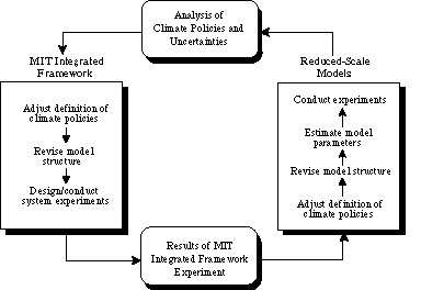
Figure 1. Interplay between the reduced-scale models and the MIT IGSM.

Proceeding around the top of the figure, the reduced-scale models can also be used to inform subsequent analyses of climate policy, using the limited number of runs that are feasible within the larger integrated framework. The reduced-scale results also indicate which uncertainties are important to policy choice. This information can, in turn, lead to a judicious selection of cases to run using the more computationally expensive parts of the IGSM. And so the analysis proceeds around the diagram, so long as the expected improvement from additional rounds is worth the cost of analysis.

In the results below, we show the first pass of such a procedure, and we indicate how the results, including sensitivity analysis of model solutions,provide inputs to the design of subsequent rounds of improvement.

Our presentation of sequential climate change decision-making is divided into three parts. In Section 2, we introduce the basic concepts that underlie our sequential modeling approach. In Section 3, we summarize the procedure by which reduced-scale system response functions are drawn from the MIT IGSM, and we formulate and explore the properties of the sequential decision model. Section 4 presents a sensitivity test of key variables treated as cerain in this application. We conclude, in Section 5, with a discussion of the policy relevance of our results and the directions they results suggest for subsequent efforts to improve the information input to climate decisions and negotiations.

2. SEQUENTIAL CLIMATE CHANGE DECISION-MAKING

Viewing climate change as a problem of sequential decisions under uncertainty highlights the fact that the preferred course of action at any particular point in time will depend, in part, upon the choices available at subsequent decision points, and on what might be learned along the way about potential climate change. Also, both mid- and long-term abatement choices may depend on the observed outcomes of short-term policy actions. Such a decision context, where decisions and information unfold sequentially, is a dynamic programming problem, and various algorithms exist for determining the optimal policy associated with this type of problem formulation.

Such problems are most commonly formulated as decision trees, and are solved by backward induction. Here we apply an alternative formulation--whose solution is also grounded in dynamic programming--which uses influence diagrams (IDs).[4] The influence diagram is both visually efficient and computationally powerful, and is a particularly useful method when a decision tree representation may have so many nodes and branches that it is easy to get lost in the forest. To provide background for the discussion below, we begin with a summary of the notation and concepts that underlie this way of laying out a choice situation.

2.1 Influence Diagrams: Concepts and Notation

IDs are graphical networks designed to represent the important qualitative features of key elements of a decision problem. The flow of information, and its functional relation to choices of action, can be displayed to any desired level of aggregation. Most real-world decision problems are formulated in a domain consisting of decision variables D = {D₁,..., D_m} and uncertain quantities U = {X₁,..., X_n}; the ID provides a convenient means for representing the relationships among these components.

Formally, an ID is a directed acyclic graph whose vertices or "nodes" represent either decision variables, random variables, or value functions:

* Decision Nodes. Represent actions under the full control of the decision-maker, and are depicted graphically as squares ;

* Chance Nodes. Represent the random or uncertain variables, and are depicted graphically as circles or ovals ;

* Value Nodes. Represent some key quantity or value resulting from decisions made or associated with a particular state of nature; depicted graphically as diamonds or rounded squares ,

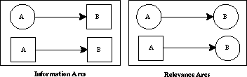
Figure 2. Information and relevance arcs in influence diagrams.

Identifying "relevance" is an important task in the construction of an ID. We begin by ordering the variables in U = (X₁,...,X_n), and for each variable X_i, specify a set of parents,par(X_i) {X₁,...,X_i-1, D}, such that

Pr {X_i | X₁,...,X_i-1, D} = Pr {X_i | par(X_i)}. (1)

The construction of an ID requires that, for every variable z par(X_i), we place a relevance arc from z to X_i in the diagram.

Following this procedure, associated with each chance node X_i in an ID are the probability distributions Pr{X_i | par(X_i)}. The so-called "chain rule" of probability states that

Pr {X₁,..., X_n | D} = Pr {X_i | X₁,...,X_i-1, D}. (2)

Given Eqs. 1 and 2, it follows that any ID for U D uniquely determines the following joint probability distribution for U given D [2]:

Pr {X₁,..., X_n | D} = Pr {X_i | par(X_i)}. (3)

In this way, IDs provide a quantitatively rigorous basis for providing a complete probabilistic description of decisions under uncerainty. During the course of the past decade, a number of numerical procedures have been developed for computing the optimal decision policy from an ID.[5]

2.2 Illustration

The ID modeling language can be illustrated using the landmark study by Manne and Richels [10], which presents a framework for dealing with uncertainty in assessing CO₂ emission reduction strategies. Their two-period,"Act-then-Learn" formulation assumes that decisions concerning CO₂ emission reductions are made at two discrete points in time, twenty years apart. As illustrated in the schematic decision tree in Figure 3, energy sector supply and demand decisions for the period 2000-2020 are made prior to knowing the damage potential of global climate change. They further assume that the damage potential is characterized by three possible states of nature: `Low,' `Moderate,' and `High.' At the second point in time, there is, in principle, a choice of action based on observation of evidence over the period 2000 to 2020. They assume a "best" CO<sub>2</sub> emission reduction level for each of these three possible states of nature. If, for example, the damage potential is `Low,' then, from 2020 on, no limits are imposed on global carbon emissions. Alternatively, the `Moderate' and `High' damage potentials give rise to assumed carbon emission reductions of 20% and 50% below 1990 levels,respectively. By assigning a subjective probability distribution to the damage potential, the model is used to evaluate an optimal hedging policy for 2000 and 2020, without knowing which carbon emission scenario will obtain.[6]

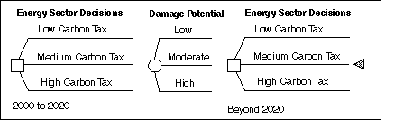
Figure 3. Act-then-learn decision framework of Manne and Richels [10].

In Figure 4, we represent the Manne-Richels model formulation as a temporal influence diagram (TID). The boxes indicate the decisions at the two stages, and the directed arc between them--a so-called "no-forgetting" arc--introduces a time ordering into the diagram. Each of the decisions brings some level of abatement cost (which, in their model formulation, includes both climate damages and emissions mitigation costs), represented by the two value nodes. The one uncertainty is the damage potential associated with global climate change, which is resolved at the end of Period 1. In this way,information concerning the damage potential is taken into account in the decision made at the beginning of Period 2.

Figure 4. Temporal influence diagram representation of the act-then-learn decision framework of Manne and Richels [10].

While formulations like that of Manne and Richels are useful and transparent pedagogical devices, our proposed framework is designed to move a step closer to the salient features and details of the problem, using relations fitted to the MIT modeling system. In the following section, we set forth an integrated decision analysis (IDA) framework for evaluating sequential abatement policies under uncertainty.

3. A SEQUENTIAL DECISION MODEL

3.1 Influence Diagram Representation

Our sequential model formulation begins with the TID shown in Figure 5. We provide a brief summary of its structure before describing it in detail. The diagram depicts a two period model, covering the years 2000-2010 and 2010-2050, with a no-forgetting arc to indicate the time ordering of the two abatement decisions. Decisions in each period lead to abatement costs (here representing the costs of emissions control in each period), and to changes in global mean surface temperature. Both abatement costs and temperature change are represented as value nodes. Temperature changes lead to impacts (a value node), which, when combined with abatement costs, yields the aggregate social loss in each period (also a value node). Note the parallel structure of decision and value nodes in Periods 1 and 2, with the graph rotated top-to-bottom in Period (2), so as to highlight the uncertainties that apply to both periods of the model.

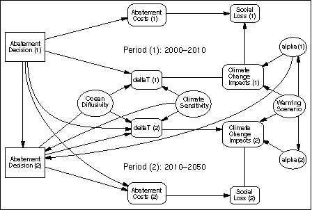
Figure 5. Temporal influence diagram representation of the sequential decision model.

In our model formulation, global climate change is represented as a dynamic process that is functionally dependent on (i) the abatement decision in each period, and (ii) chance variables representing the uncertainty characterizing two important climate-related parameters: climate sensitivity and ocean diffusivity. Stated in this way, key uncertainties in the climate system are characterized and represented in terms that are familiar to scientists working in the field. Also, the impacts associated with climatic change are subject to uncertainty. In the example presented here, the costs of emissions abatement are treated as certain.[7] The directed arcs from the uncertain quantities Climate Sensitivity and Ocean Diffusivity to Abatement Decision (2), but not to Abatement Decision (1), show that, for the purposes of our analysis here, we assume that uncertainty concerning the response of the climate system is resolved at the end of Period 1, i.e., before the Period 2 decision is made. Similarly, we assume that uncertainty concerning the parameterization of the damage function associated with Period 1 is resolved at the end of that period.

The TID in Figure 5 provides a computationally-efficient framework for exploring sequential climate policies. In its 1996 report, the IPCC notes that,"the intractability of complex decision trees has limited the application of [decision analysis] in environmental problems..." [3, p. 67]. To emphasize this point, we note that--for the sequential decision basis that we specify below--the decision tree equivalent for the TID in Figure 5 contains over one thousand end points. Needless to say, trees of this complexity are computationally intractable, and are of little use as communication devices. We believe that ID-based methodology facilitates communication with both experts and non-experts, alike.

In what follows, we formally specify the sequential decision basis for the TID described above. We use quantified expert judgements to estimate the economic impact of climatic change, and to specify subjective probability distributions for key climate-change-related quantities and model parameters.[8] Wherever possible, we have drawn from published elicitations and surveys of expert opinion, most notably, Morgan and Keith [13] and Nordhaus [14].

3.2 Specification of the Sequential Decision Basis

3.2.1 Sequential Decision Alternatives

We assume a single decision-maker who must choose among a finite set of possible abatement strategies, applied over the two-periods of the decision model.[9] We focus on the selection of optimal sequential decision strategies, for the two decision nodes, Abatement Decision (1) and Abatement Decision (2). For i = 1, 2, we define both of these decision nodes as follows:

Abatement Decision (i) = {a_i1,a_i2, a_i3,a_i4},
where
a_i1 = Reference Baseline-No Controls;
a_i2 = Stabilize OECD Carbon Emissions at 1990 Levels;
a_i3 = AOSIS-Like Protocol;
a_i4 = Stringent Abatement.

Abatement decisions a₁₁ and a₂₁ represent an unconstrained `Reference' carbon emission baseline. Abatement costs are defined as the difference in costs between the Reference baseline scenario and policy scenarios where carbon emissions are constrained. Under abatement decisions a₁₂ and a₂₂, OECD carbon emissions are stabilized at 1990 levels. Abatement decisions a₁₃ and a₂₃ represent a protocol similar to that proposed by the Alliance of Small Island States (AOSIS) and Germany [1]. In our version of the AOSIS proposal, OECD countries agree to reduce CO₂ emissions to 20% below 1990 levels by the year 2005[10] and there are no commitments to reduction or limitation of GHG emissions by non-OECD countries. Finally, under abatement decisions a₁₄ and a₂₄, OECD carbon emissions are reduced to 30% of 1990 levels.

Figure 6 uses a schematic decision tree to depict the abatement decisions described above, showing the 16 possible decision sequences. We formally denote a sequential climate policy by the ordered pair,<a_1i, a_2j>, where a_1i Abatement Decision (1) and a_2j Abatement Decision (2). An abatement decision adopted at the beginning of Period 1 can be revised at the beginning of Period 2. If in Period 1, for example, abatement decision a₁₂ is adopted, then in Period 2, the decision-maker can (i) abandon the decision and adopt a no-controls policy (Abatement Decision a₂₁); (ii) continue with the adopted policy (Abatement Decision a₂₂); or (iii) adopt a more stringent policy (Abatement Decision a₂₃ or a₂₄). Also, the formulation includes an explicit representation of delayed policy action, by means of sequential climate policies <a₁₁,a₂₂>, <a₁₁, a₂₃>, and <a₁₁, a₂₄>.

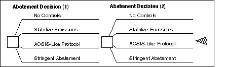
Figure 6. Schematic decision tree for the two-period model.

3.2.2 Representation of Possible States of the Climate System

The magnitude of climate change, stated in terms of changes in global mean surface temperature in 2010 and 2050 is, in Figure 5, labeled deltaT (1) and deltaT (2). As described earlier, these two value nodes depend on the abatement action, and on the state of nature concerning the response of the climate system to GHG emissions. Two variables are used here to summarize the uncertainty about this aspect of the climate system: Climate Sensitivity and Ocean Diffusitivity. Climate sensitivity represents the response of the atmospheric system to radiative forcing, assuming the system is in equilibrium with the ocean. Ocean diffusivity represents the role of ocean circulations in sequestering heat, thereby delaying the realized temperature change in the lower atmosphere.

In keeping with our approach, which involves estimating key reduced-form model parameters from the larger MIT integrated framework, these variables are specific to the climate portion of the IGSM formulation.[11] Several phenomena influence climate sensitivity,including surface albedo, water vapor feedback, and cloud effects. The dominant uncertainty concerns cloud effects, and it is through a cloud parameter that uncertainty is imposed in the model. Resulting model response is stated in terms of the familiar definition of climate sensitivity, which is the equilibrium response to doubled CO₂ concentration. The ocean model now implemented in the IGSM contains a diffusion approximation of ocean circulations, and the parameter tested here is the key one determining their strength.

The uncertain quantities Climate Sensitivity and Ocean Diffusitivity are assumed to take on a finite number of possible states, which we define as follows:

Climate Sensitivity = {Low, Medium, High},
where
Low = 1.5^oC;
Medium = 2.5^oC;
High = 4.5^oC;
and
Ocean Diffusitivity = {od₁, od₂, od₃,od₄},
where
od₁ = 1/50;
od₂ = 1;
od₃ = 1;
od₄ = 1;

These states of the climate system, combined with the sequence of abatement decisions, yield a model of global climate change as a dynamic process.

The TID in Figure 5 asserts that Climate Sensitivity and Ocean Diffusitivity are probabilistically independent, and thus can be assessed separately.[12] The probability distribution for Climate Sensitivity is specified as follows: `Low' and `High' are each assigned probabilities of 0.2, and `Medium' is assigned a probability of 0.6. For Ocean Diffusitivity, od₂ and od₃ are assigned probabilities of 0.6 and 0.199, respectively; od₁ and od₄ are assigned probabilities of 0.2 and 0.001, respectively.

For each abatement policy a_1i Abatement Policy (1), the functional dependence shown in Figure 5 of deltaT (1) on Climate Sensitivity and Ocean Diffusivity gives rise to a value node data structure of the form depicted in Figure 7. Note that the deltaT (1) value node is defined in terms of twelve separate projections of global-mean surface temperature change, one for each possible Climate Sensitivity-Ocean Diffusivity pair. The data structure for deltaT (2) is identical to that of deltaT (1), only the structure is conditioned by the abatement policy choices made in both Periods 1 and 2; the dual conditionality arises from the presence of the no-forgetting arc between the TID's two decision nodes.

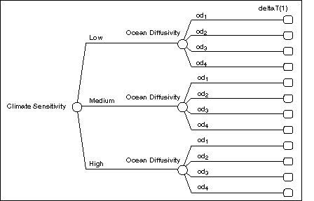
Figure 7. Data structure for the deltaT(1) value node, conditioned by the selection of an abatement policy a_1i Abatement Policy (1).

In order to numerically specify the data structures corresponding to the deltaT (1) and deltaT (2) value nodes, we utilize the following globally-averaged one-box climate model:[13]

t_t = t_t-1 + C₁ (Climate Sensitivity, Ocean Diffusivity) [F_t-1 - lt_t-1]. (3)

This structural specification is, in effect, the reduced-scale or "nimble" version of the climate model discussed above, and whose use is illustrated in Figure 1. For the purposes of the analysis presented here, we calibrate this model to transient simulations of the MIT 2D-LO global climate model. As described by Valverde [24], the calibration procedure utilizes econometric and statistical time series estimation techniques to obtain a range of estimates for the inertial parameter, C₁, which in Eq. 3 is shown to be a function of Climate Sensitivity and Ocean Diffusivity. For the possible states of nature defined above, we obtain twelve separate estimates for the inertial parameter. These twelve estimates give rise to an equal number of numerical specifications for Eq. 3.

Numerical implementation of Eq. 3 requires that we provide an exogenously-specified radiative forcing time series, . For a given radiative forcing trajectory, the twelve numerical specifications for Eq. 3 give rise to twelve projections of global-mean surface temperature change, for times t = 1,...,T. In our TID, for each sequential climate policy, < a_1i, a_2j>, we therefore assess a corresponding radiative forcing trajectory, . As illustrated in Figure 8, we apply elements of the MIT IGSM to assess the radiative forcing time-paths and, as we discuss below, the abatement costs associated with each of the sixteen sequential climate policies outlined above.

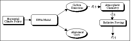
Figure 8. Linkages between the IDA framework, the MIT IGSM, and the reduced-scale global climate model(s).

Using Eq. 3, for each radiative forcing trajectory, , we compute twelve separate projections for deltaT (1) and for deltaT (2). As part of our sequential analysis, we tabulate the global carbon emission,atmospheric CO₂ concentration, and radiative forcing time-paths associated with each sequential climate policy. We must also tabulate, for each of the sixteen sequential climate policies, the one-box climate model projections for deltaT (1) and deltaT (2), as a function of Climate Sensitivity and Ocean Diffusivity.

3.2.3 Sequential Abatement Costs

The economic costs associated with each sequential climate policy are measured in terms of percentage loss of gross domestic product (GDP). In our primary TID, abatement costs in each period are represented numerically in the form of a value node data structure, with values drawn from output of the MIT Emissions Prediction and Policy Analysis (EPPA) model, which is a component of the IGSM.[14] EPPA is a global, computable,general equilibrium model that projects anthropogenic GHG emissions based on analysis of economic development and patterns of technical change. In Table 1, we summarize the Period 1 and Period 2 abatement costs associated with each sequential climate policy, < a_1i,a_2j >. The costs are stated in terms of percentage of GDP loss for the periods 2000-2010 and 2010-2050, assuming a 5% discount rate. In these sample calculations, it is assumed that there is no trading in emissions permits.

Table 1. Abatement costs incurred in Periods 1 and 2, for each sequential climate.

Sequential Climate Policy	Abatement Cost (1)	Abatement Cost (2)
<a11,a21>		0%
<a11, a22>		0.84%
<a11,a23>	0%	1.16%
<a11,a24>		1.49%
<a12,a21>		0.15%
<a12,a22>		0.84%
<a12,a23>	0.32%	1.23%
<a12,a24>		1.47%
<a13,a21>		0.25%
<a13,a22>		1.04%
<a13,a23>	0.45%	1.43%
<a13,a24>		1.67%
<a14,a21>		0.32%
<a14,a22>		1.11%
<a14,a23>	0.55%	1.48%
<a14,a24>		1.78%

3.2.4 Specification of Climate Change Impacts

The literature on the economic valuation of climate change impacts is at an early stage of development,[15] and the MIT IGSM does not yet produce a summary measure of climate-change effects at the level needed for the type of analysis considered here. We therefore adopt an approach to damage valuation similar to that used by Nordhaus [15], Peck and Teisberg [18], and others. Specifically, we are interested in specifying a damage function, D, whose domain is defined as the level or magnitude of climate change at time t.

Frequently the damage function is assumed to take the form

D(t_t) = (t_t)^g, (4)

where, as before, t denotes the change in global-mean surface temperature at time t, and g characterizes the order of the damage function. The parameter g is usually assumed to take on the values 1, 2, or 3.[16] Unfortunately, use of this equation can give rise to counter-intuitive or pathological results. An implied assumption is that larger values of the parameter g necessarily entail larger damages. If, however, the temperature change over some finite time period is less than 1^oC, then it follows that (t_t) > (t_t)² > (t_t)³, in which case welfare loss is seen to decrease with increases in the order of the damage function.

To avoid this potential pitfall, we characterise the damages in each of the two periods of the decision model by an exponential function of the form

D(t_t) = e^at_t - 1 (5)

where t_t is defined as before, and a is a scaling constant. For any two values a₁ < a₂, it follows that e^a1tt < e^a2tt, for all positive values of t_t.

Typically, damage functions such as Eqs. 4 and 5 are calibrated so that, for particular levels of global-mean surface temperature change, damages are seen to equal a certain percentage of gross production. Peck and Teisberg [18], for example, assume that the damage associated with a 3^oC surface temperature rise is 2% of gross production--a value which they refer to as the adaptation/damage percent. [17]

In this analysis, rather than assume a single deterministic specification for Eq. 5, we treat the calibration and parameterization of this damage function as uncertain in the decision model. Specifically, rather than anchoring Eq. 5 to a single level of climatic change (e.g., 3^oC), we calibrate the damage function against two climate change scenarios, one characterized by a low level of warming and the other characterized by a high level. For each warming scenario, we utilize quantified expert judgement to specify `Low,' `Medium,' and `High' estimates for the expected adaptation/damage percent in the sequential model's two periods.

The two warming scenarios applied in the calibration of Eq. 5 are drawn from the one-box climate model projections for global-mean surface temperature change under the Reference baseline scenario. In particular, for the low warming scenario, we select the low values for deltaT (1) and deltaT (2) under sequential climate policy <a₁₁, a₂₁>; similarly, for the high warming scenario, we select the high values for deltaT (1) and deltaT (2) under the same sequential policy. For the analysis presented here, the temperature change projections for the low warming scenario are 0.470^oC and 0.876^oC for Periods 1 and 2, respectively; the corresponding temperature change values for the high warming scenario are 1.340^oC and 2.913^oC.

An expert judgement elicitation of the expected adaptation/damage percentages associated with the low and high warming scenarios yields an illustrative set of values such as those shown in Table 2.[18] The `Low,' `Medium,' and `High' percentages associated with each warming scenario are interpreted as the 0.05, 0.50, and 0.95 fractiles of a cumulative probability distribution for the expected adaptation/damage percent in each period. For each row of values in Table 2, we solve Eq. 5 for the corresponding `Low,' `Medium,' and `High' values of the scaling parameter, a. We summarize these values in Table 3. Using these calibrated parameter values,in Figures 9 and 10 we plot the damage functions associated with the low and high warming scenarios, respectively, for Periods 1 and 2.

Table 2. Low, medium, and high estimates for the expected adaptation/damage percentages associated with the low and high warming scenarios.

	Expected Adaptation/Damage Percent
Low Warming Scenario	Low	Medium	High
0.470oC rise by 2010	0.1%	0.75%	1%
0.876oC rise by 2050	0.2%	1.75%	3%
High Warming Scenario	Low	Medium	High
1.340oC rise by 2010	0.2%	2.25%	4%
2.913oC rise by 2050	0.3%	3.75%	10%

Table 3. Calibrated low, medium, and high values for the damage function scaling parameter, a.

	Calibrated Scaling Parameter a
Low Warming Scenario	Low	Medium	High
0.470oC rise by 2010	0.203	1.191	1.475
0.876oC rise by 2050	0.208	1.155	1.583
High Warming Scenario	Low	Medium	High
1.340oC rise by 2010	0.136	0.880	1.201
2.913oC rise by 2050	0.090	0.535	0.881

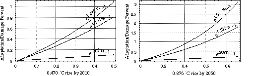
Figure 9. Damage functions for the low warming scenario, for Periods 1 and 2 of the sequential decision model.

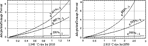
Figure 10. Damage functions for the high warming scenario, for Periods 1 and 2 of the sequential decision model.

As mentioned earlier, we treat the calibration and parameterization of the damage functions shown in Figures 9 and 10 as uncertainties in the model. In particular, consistent with our discussion above, we define a chance node

Warming Scenario = {Low, High},

where

Low =

High =

As before, we specify a discrete subjective probability distribution for this chance variable. The nominal values used for the distribution are as follows: the `Low' warming scenario is assigned a probability of 0.7, and the `High' warming scenario is assigned a probability of 0.3.

In our primary TID, the chance node Warming Scenario is seen to condition two chance nodes, alpha (1) and alpha (2), each defined in terms of three possible states of nature, corresponding to the `Low,' `Medium,' and `High' values of the calibrated scaling parameter, a. Also, the chance nodes alpha (1) and Warming Scenario have directed arcs that lead into a value node labeled Climate Change Impacts (1); similarly, alpha (2) and Warming Scenario have directed arcs that lead into a value node labeled Climate Change Impacts (2). This set of functional specifications give rise to a pair of value node data structures--illustrated in Figure 11--for representing climate-change-related impacts.

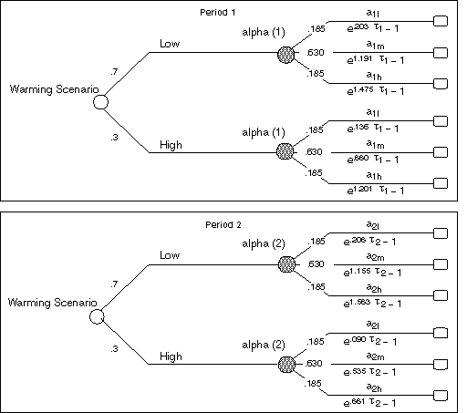
Figure 11. Data structures for the Climate Change Impacts (1) and Climate Change Impacts (2) value nodes.

In specifying probability distributions for alpha (1) and alpha (2), we simplify the assessment procedure by assuming that these two chance nodes are conditionally independent, given Warming Scenario. In addition, the directed arcs from Warming Scenario to alpha (1), and from Warming Scenario to alpha (2), are--for our purposes here--interpreted as non-conditioning arcs. As described earlier, the `Low,' `Medium,' and `High' values of the scaling parameter, a, are interpreted as the 0.05, 0.50, and 0.95 fractiles of a cumulative probability distribution function. In specifying these distributions, we use the extended Pearson-Tukey method to obtain a three-point approximation. The resulting `Low,' `Medium,' and `High' values of the chance nodes alpha (1) and alpha (2) are assigned probabilities of 0.185, 0.63, and 0.185, respectively.

3.2.5 Aggregating Abatement Costs and Climate Change Impacts

In the TID shown in Figure 5, abatement costs and climate change impacts are aggregated in each period via the following set of equations:

Social Loss (1) = Abatement Costs (1) + Climate Change Impacts (1);

and

Social Loss (2) = Abatement Costs (2) + Climate Change Impacts (2).

3.3 Evaluation of the Model

Having specified the sequential decision basis for our model, the TID in Figure 5 can now be evaluated to determine the optimal sequential climate policy. Recall that uncertainty concerning Climate Sensitivity, Ocean Diffusivity, and alpha (1) is assumed to be resolved prior to choosing an optimal GHG abatement policy in Period 2. As shown in Table 4, the expected social loss associated with our sequential decision model is 5.70%. Also summarized in this table are the policy prescriptions of the model. In Period 1, the optimal course of GHG abatement action is to pursue policy a₁₁, i.e., a `No Controls' policy.[19] Thus, in the center panel of Table 4, we see that for Abatement Decision (1), the probability associated with policy a₁₁ is 1.0. The right-hand panel of Table 4 shows that the abatement policies in Period 2 have probabilities that, together, sum to 1.0. The reason is that in Period 2, the optimal choice depends on the outcomes of the chance events Climate Sensitivity, Ocean Diffusivity, and alpha (1). These probabilities reflect the likelihood that a particular policy choice will be made, if the optimal policy is followed; we shall refer to this likelihood as a probabilistic climate policy.

The results in Table 4 immediately suggest one direction for subsequent stages of the analysis, using the iterative procedure in Figure 1. The solution in Table 4 indicates a low probability of ever choosing one of the more stringent abatement levels, and that a substantial change in assumptions would be needed to move the optimal Period 1 choice from No-Controls (Abatement Decision a₁₁) to 1990 Stabilization (Abatement Decision a₁₂). Given the economic growth between 1990 and 2010, the degree of abatement in 2010 is near 30%, if measured from the No-Controls case. This suggests that our next step would be to reformulate the decision set (adding a case intermediate between the No-Controls and 1990 Stabilization, and perhaps reducing the severity of the Stringent Abatement option) in order to explore more fully the region where the optimal policy seems to lie.

Table 4. Probabilistic climate policies for the sequential model.

	Probabilistic Climate Policies
Expected Social Loss	Abatement Decision (1)		Abatement Decision (2)
	a11	1.0	a21	0.54
5.70%	a12	0	a21	0.432
	a13	0	a21	0
	a14	0	a21	0.028

This change would then require re-estimation of cost data within the EPPA sub-model of the IGSM--a move through the Figure 1 circuit.

There is a further interpretation of these results that enables us to form a judgement about the validity of the sequential decision analysis itself. The Period 1 abatement choice a₁₁ (no-controls) is optimal only if, when the relevant uncertainties are resolved, the second stage decision that turns out to be best is actually followed. If this proposition is not credible, then the analysis, and its recommendation for the Period 1 choice,are not correct. The results in Table 4 show that it is highly unlikely that a cutback as stringent as the AOSIS proposal will be called for in Period 2. On the other hand, there is a probability of over 0.4 that the stabilization policy will appear optimal at the beginning of Period 2, and one has to believe that this policy is politically feasible at that time (a factor outside the analysis as formulated here) for the recommendation of policy a₁₁ to have validity, even within the narrow definition of the decision set as formulated here.

4. SENSITIVITY ANALYSIS

Sensitivity analyses can be used to test the robustness of the sequential model's policy prescriptions, as well as to provide additional information for guiding subsequent stages in the iterative analysis procedure. One such application is illustrated here, to explore the implications of our having treated abatement costs as certain, when in fact they are not. Recall that each of the sixteen sequential climate policies considered here is characterized by a pair of abatement costs (obtained from the MIT EPPA model), one for each of the two periods in the model. We analyse the sensitivity of the sequential decision model's expected value and policy prescription to changes in the numerical values specified for Abatement Costs (1) and Abatement Costs (2). The range of values utilized for this analysis is shown in Table 5. The Period 1 costs span a roughly three-fold variation between low and high extremes; the Period 2 values reflect a roughly 1.5-fold variation.

Table 5. Range of abatement costs incurred in Periods 1 and 2, for each sequential climate policy.

Sequential	Abatement Costs (1)			Abatement Costs (2)
Climate Policy	Low	Nominal	High	Low	Nominal	High
<a11,a21>					0
<a11,a2>		0		0.67%	0.84%	1.02%
<a11,a23>				0.93%	1.16%	1.39%
<a11,a24>				1.19%	1.49%	1.78%
<a12,a21>				0.12%	0.15%	0.18%
<a12,a22>	0.16%	0.32%	0.48%	0.67%	0.84%	1.02%
<a12,a23>				0.98%	1.23%	1.48%
<a12,a24>				1.18%	1.47%	1.76%
<a13,a21>				0.2%	0.25%	0.3%
<a13,a22>	0.23%	0.45%	0.68%	0.83%	1.04%	1.25%
<a13,a23>				1.14%	1.43%	1.72%
<a13,a24>				1.34%	1.67%	2.02%
<a14,a21>				0.26%	0.32%	0.38%
<a14,a22>	0.28%	0.55%	0.83%	0.89%	1.11%	1.33%
<a14,a23>				1.18%	1.48%	1.78%
<a14,a24>				1.42%	1.78%	2.14%

Using these low and high values, we can construct a series of value sensitivity comparisons showing which components of the decision problem are most affected by these assumptions for Abatement Costs (1) and Abatement Costs (2). A helpful way to display the results is in the form of a horizontal bar graph showing the changes in expected value induced by varying one or another of these inputs across its assumed range, while holding all other input parameters at their reference values. If the bars are sorted top-to-bottom in order of relative impact, the result is the "tornado" diagram shown in Figure 12. The expected value of the original model is shown by the line at 5.70%. As the figure shows, the most important of the cost variations imposed in this sensitivity test is Abatement Costs (2) for sequential climate policy <a₁₁, a₂₂>. Of lesser importance is the influence of the Period 2 cost ranges for policies <a₁₁, a₂₃> and <a₁₁, a₂₄>.

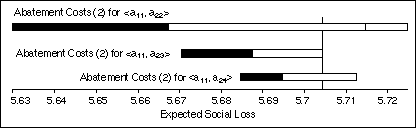
Figure 12. Tornado diagram for Abatement Costs (1) and Abatement Costs (2).

The remaining low and high values specified for Abatement Costs (1) and Abatement Costs (2) have no influence on the expected value of the model (so no bars are shown for these cases).

In Figure 12, shifts away from the nominal model's optimal policy are indicated by changes in shade. In our two-period model formulation, as each model value traverses its specified low-high range, there are four possible outcomes for the optimal sequential climate policy:

1. There is no change in the optimal abatement policy in Period 1 and,similarly, no change in the probabilities associated with the Period 2 policy options;

2. There is no change in the optimal abatement policy in Period 1, but there are changes in the probabilities associated with the Period 2 abatement options;

3. There is a shift in the optimal abatement policy in Period 1, but no changes in the probabilities associated with the Period 2 policy options;

4. There are shifts in both the optimal Period 1 policy, and in the probabilities associated with the Period 2 options.

Figure 13 plots the Period 2 probabilistic climate policies that are obtained by evaluating the decision model at each of the five points in the range 0.67% to 1.00% where shifts in optimal policy occur. Also included in this plot are the Period 2 probabilities associated with our nominal model specification (presented earlier in the right-hand panel of Table 4). Figure 13 reveals some interesting characteristics of these sets of probabilistic climate policies. Note, first, that as Abatement Costs (2) for climate policy <a₁₁, a₂₂> increase across the specified range of values, so too does the probability associated with abatement policy a₂₁. Specifically, as Abatement Costs (2) for <a₁₁, a₂₂> is varied between roughly 0.70% to 0.866%, we observe a gradual increase in the probability associated with policy a₂₁ (from 0.512 to 0.552). However, as the abatement cost shifts from 0.866% to 0.869%, the probability of policy a₂₁ jumps from 0.552 to 0.804. Note, also, that as we traverse the range of values from 0.70% to 0.95%, the probability associated with policy a₂₂ decreases from 0.460 all the way down to 0. These sensitivity results are significant for several reasons. First,recognizing that policy a₂₂ represents the least stringent abatement option considered here (with the exception, of course, of the Reference baseline policy, a₂₁), it is interesting to note that, as we traverse upwardly the specified range of values for Abatement Costs (2) under climate policy <a₁₁, a₂₂>,we move from a situation where the odds associated with adopting some level of abatement action are roughly even, to a situation where abatement action of any kind becomes increasingly unlikely.

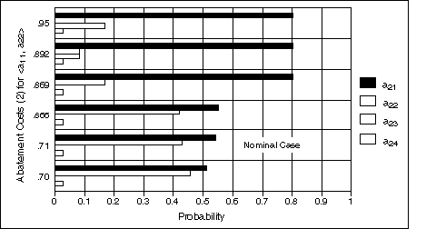
Figure 13. Probabilistic climate policies for Period 2, as a function of six different values for Abatement Costs (2) under sequential climate policy <a₁₁, a₂₂>.

Looking, briefly, at the other probabilistic climate policies shown in Figure13, we note that as Abatement Costs (2) for climate policy <a₁₁, a₂₂> go from roughly 0.70% to 0.869%, abatement policy a₂₃ is never an optimal course of action, i.e., the probability of adopting this course of action is, for the particular range of values explored here, zero. If Abatement Costs (2) for this policy rise as high as 0.892%, then policy a₂₃ is a live prospect. Alternatively, looking at policy a₂₄, we note that the probability associated with this response option remains fixed at 0.028, across the entire range of values considered here.

Clearly, in the sample climate decision studied here the overall analysis task was simplified by treating emissions control costs as known with certainty. These sensitivity calculations illuminate the question whether the decisions that are the focus of the exercise are likely to be changed if cost uncertainty is introduced in subsequent rounds of the analysis. For this example, the Period 1 choice is not sensitive to the assumed variation in cost, though the probability that substantial controls must be anticipated in Period 2 is affected. Of course, with a redefinition of the choice set to gain better discrimination at lower levels of control, cost uncertainty would likely have greater impact. In this way, sensitivity analysis can play an important role not just in interpreting results but in the process formulation illustrated in Figure 1.

5. CONCLUSIONS

The analytical framework presented here provides policy analysts and decision-makers with a nimble, computationally-efficient vehicle for evaluating a broad range of possible GHG abatement policies under uncertainty. The sequential model formulation integrates a reduced-scale approach to climate modeling and prediction, with the analysis linked to a specific larger modeling framework, in this case the MIT Integrated Global System Model. The proposed approach facilitates the process of expert elicitation, which is needed in analyses of this kind. It also supports a clear, iterative approach to estimation and numerical specification of reduced-scale models, allowing efficient use of large-model computer runs, and it provides a clear basis for checking and documenting results. This approach of fitting to a specific larger system is, of course, generalizable, and can be applied to other integrated assessment efforts. Indeed, such analysis should be done more generally,because the results would reveal much about the differences among models values imposed in the type of decision context considered here.

Further, several important aspects of sequential decision problems, which may difficult to communicate otherwise, are made more transparent using the approach applied here. As with previous applications to climate policy over time, the analysis shows the "best" choice today, given the choices considered,and the underlying models. Furthermore, it also makes clear that, even with a recommendation for today's choice, the preferred future choice (in Period 2, in the example presented here) can only be computed with some probability. Since the optimality of the current choice only holds if it can be said with certainty that the decision that ultimately becomes optimal in the later period will actually be taken, the notion of a probabilistic climate policy (Table 4) is important information in judging whether this key assumption is supportable.

As with other methods, our IDA framework supports analysis of the sensitivity of the expected value of the sequential choice problem, and the specific decisions in each period, to uncertainties that are not treated explicitly in the analysis (e.g., abatement costs, in the example used here). These sensitivity studies are an important component of the sequential estimation procedure described in Section 1, for they can guide the design of subsequent runs of the parent framework to focus on regions of variables where there is the greatest influence on decisions. Without the iterative procedure shown in Figure 1, the choice of underlying large-system runs is largely a matter of guesswork.

Many lines of fruitful work lead from the formulation and example policies presented here. Important additional insights can be gained from formulations that take explicit account of uncertainty in emissions forecasts and abatement costs. More challenging, but nonetheless useful, extensions include the ability to take account of less than complete resolution of key uncertainties, and less than complete certainty that the future choices implied by the optimal solution can and will be carried out. But even without these improvements, this form of analysis should help clarify the nature of choices faced in the climate area and, one hopes, lead to more coherent policy discussions.

ACKNOWLEDGEMENTS

This research was funded by the U.S. National Oceanic and Atmospheric Administration (NA56GP0376). The MIT Integrated Global System Model used in the work has been developed with the support of a government-industry partnership including the U.S. Department of Energy (901214-HAR; DE-FG02-94ER61937; DE-FG02-93ER61713), U.S. National Science Foundation (9523616-ATM), and U.S. Environmental Protection Agency (CR-820662-02), the Royal Norwegian Ministries of Energy and Industry and Foreign Affairs, and a group of corporate sponsors from the United States, Europe and Japan. The authors thank Andrei Sokolov for assistance with the key components of the MIT modeling system, and Caroline Rudd for assistance in the preparation of this document.

REFERENCES

[1] Draft Protocol to the United Nations Framework Convention on Climate Change on Greenhouse Gas Emission Reduction. United Nations Framework Convention on Climate Change, 1994.

[2] R.E. Barlow. Using influence diagrams. In: Accelerated Life Testing and Experts' Opinions in Reliability, C.A. Clarotti and D.V. Lindley, editors,pp. 145-157. North-Holland Physics Publishing, 1988.

[3] J. Bruce, H. Lee, and E. Haites, editors. Climate Change 1995: Economics and Social Dimensions of Climate Change. Cambridge University Press, New York, 1996.

[4] Robert T. Clemen. Making Hard Decisions: An Intorduction to Decision Analysis. Duxbury Press, Belmont, California, second edition, 1996.

[5] Hadi Dowlatabadi. Integrated assessment models of climate change: An incomplete overview. Energy Policy, 23(4-5):289-296, 1995.

[6] Hadi Dowlatabadi and M. Granger Morgan. A model framework for integrated studies of the climate problem. Energy Policy, pp. 209-221, March,1993.

[7] James K. Hammitt, Robert J. Lempert, and Michael E. Schlesinger. A sequential-decision strategy for abating climate change. Nature,357:315-318, 1992.

[8] Henry D. Jacoby et al. CO₂ emissions limits: Economic adjustments and the distribution of burdens. The Energy Journal,18(3):31-58, 1997.

[9] Alan S. Manne. Hedging strategies for global carbon dioxide abatement: A summary of poll results EMF 14 Subgroup--Analysis for decisions under uncertainty. In: Climate Change: Integrating Science, Economics, and Policy, N. Nakicenovic, W.D. Nordhaus, R. Richels, and F.L. Toth (editors),pp. 207-228. International Institute for Applied Systems Analysis, Laxenburg,Austria, December, 1996.

[10] Alan S. Manne and Richard G. Richels. Buying Greenhouse Insurance: The Economic Costs of Carbon Dioxide Emission Limits. MIT Press, Cambridge,Massachusetts, 1992.

[11] K.T. Marshall and R.M. Oliver. Decision Making and Forecasting. Series in Industrial Engineering and Management Science. McGraw-Hill, Inc., New York, 1995.

[12] Izhar Matzkevich and Bruce Abramson. Decision analytic networks in artificial intelligence. Management Science, 41(1):1-22, January,1995.

[13] M. Granger Morgan and David W. Keith. Subjective judgments by climate experts. Environmental Science and Technology, 29(10):468-476,1995.

[14] William D. Nordhaus. Expert opinion on climatic change. American Scientist, 82:45-51, January, 1994.

[15] William D. Nordhaus. Managing the Global Commons: The Economics of Climate Change. MIT Press, Cambridge, Massachusetts, 1994.

[16] Edward A. Parson. Integrated assessment and environmental policy making: In pursuit of usefulness. Energy Policy, 23(4-5):463-475, 1995.

[17] Judea Pearl. Probabilistic Reasoning in Intelligent Systems: Networks of Plausible Inference. Series in Representation and Reasoning. Morgan Kaufmann Publishers, Inc., San Mateo, California, 1988.

[18] Stephen C. Peck and Thomas J. Teisberg. Global warming uncertainties and the value of information: An analysis using CETA. Resource and Energy Economics, 15:71-97, 1993.

[19] Ronald G. Prinn et al. Integrated Global System Model for climate policy analysis: Feedbacks and sensitivity studies. Climatic Change,forthcoming.

[20] Stephen H. Schneider and Starley L. Thompson. Atmospheric CO₂ and climate: Importance of the transient response. Journal of Geophysical Research, 86(C4):3135-3147, 1981.

[21] Ross D. Shachter. Evaluating influence diagrams. Operations Research, 33(6), 1986.

[22] Andrei P. Sokolov and Peter H. Stone. A flexible climate model for use in integrated assessments. Climate Dynamics, 14:291-303, 1998.

[23] Ferenc L. Toth. Practice and progress in integrated assessments of climate change. Energy Policy, 23(4-5):253-267, 1995.

[24] L. James Valverde A., Jr. Uncertain Inference, Estimation, and Decision-Making in Integrated Assessments of Global Climate Change. PhD Thesis,Massachusetts Institute of Technology, 1997.

[25] Mort D. Webster. Uncertainty in future carbon emissions: A preliminary exploration. Report No. 30, MIT Joint Program on the Science and Policy of Global Change, 1997.

[26] Z. Yang et al. The MIT Emissions Prediction and Policy Analysis (EPPA) model. Report No. 6, MIT Joint Program on the Science and Policy of Global Change, 1996.

^* Sloan School of Management, Massachusetts Institute of Technology, Cambridge, MA 02139, USA

[1] For insightful discussions of climate-related integrated assessment modeling, see, e.g., Dowlatabadi [5], Parson [16], and Toth [23].

[2] See, e.g., Manne [9], Manne and Richels [10], Hammitt, Lempert and Schlesinger [7], Dowlatabadi and Morgan [6],and Nordhaus [15].

[3] See, e.g., Manne and Richels [10] and Hammitt, Lempert and Schlesinger [7].

[4] For a discussion of the mathematical theory that underlies influence diagrams, see, e.g., Barlow [2]. A recent textbook by Marshall and Oliver [11] focuses on issues of model formulation and evaluation using influence diagrams.

[5] For detailed, technical presentations of algorithms for evaluating IDs, see, e.g., Pearl [17, pp. 309-313] and Shachter [21]. Lucid and accessible presentations of these and related topics are found in Clemen [4, pp. 81-83] and Matzkevich and Abramson [12].

[6] Manne [9] reports the results of a study that compares the optimal hedging strategies of seven models participating in Energy Modeling Forum Study 14.

[7] This feature of the problem could also be treated in a problistic fashion, the additional task being the preparation of the needed input data. Recent work by Webster [25] represents one possible avenue for introducing uncertainty into the carbon emission forecasts and cost estimates that are derived from the MIT EPPA model.

[8] The climate change experts who participated in this study are all affiliated with the MIT Joint Program on the Science and Policy of Global Change.

[9] Extension to three or more periods is straightforward, but increasingly demanding from the vantage point of computation and analysis. The "single-actor" analysis, applied to what is clearly a multi-nation decision problem, is justified in that the results indicate the desired policy direction if suitable arrangements for cooperation and compensation can be negotiated. Extension of this work to a multi-party formulation is a subject of ongoing research.

[10] The AOSIS proposal applies the 20% restriction to all the countries in Annex I to the Climate Convention, which include the OECD nations (except Mexico), plus 12 so-called "economies in transition" in the former Soviet Union and Eastern Europe.

[11] For details on this component, see Sokolov and Stone [22].

[12] In doubled CO₂ experiments,the deep ocean is assumed to be at a temperature that is in equilibrium with the atmosphere. Since there is no physical process that "links" climate sensitivity and ocean diffusivity, we are able to assert that these two quantities are probabilistically independent.

[13] The globally-averaged one-box climate model used here was originally developed by Schneider and Thompson [20], and versions of it are used by Nordhaus [15] and others in several recent integrated assessments of global climate change. See Valverde [24] for an exploration of the use of a globally-averaged two-box climate model, which contains a second equation that provides a more explicit representation of the influence of the oceans.

[14] Documentation of the model is provided by Yang et al. [26]; for an application to a policy issue, see Jacoby et al. [8].

[15] A useful overview of this literature is provided by the IPCC [3, Ch. 6].

[16] See, e.g., Nordhaus [15].

[17] For the purposes of sensitivity analysis, Peck and Teisberg vary the adaptation/damage percent from 0.5% to 3.5%.

[18] The expected damages utilized here are consistent with those reported by Nordhaus [14].

[19] Note that, within the language of decision theory, the word "optimal" is a term of art, and implies only that the decision strategy is best within the boundaries of the defined problem. In the illustration used in this paper, for example, the `No-Controls' option that is "optimal" in Period 1 could well be inferior to a level of control somewhere between `No-Controls' and `1990 Stabilization,' but was not defined in this case.

| Top of page | | |