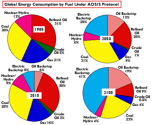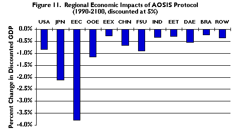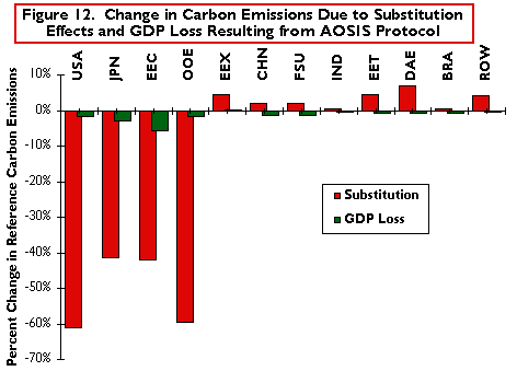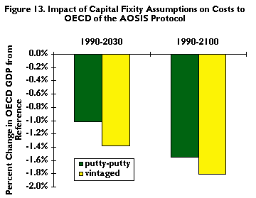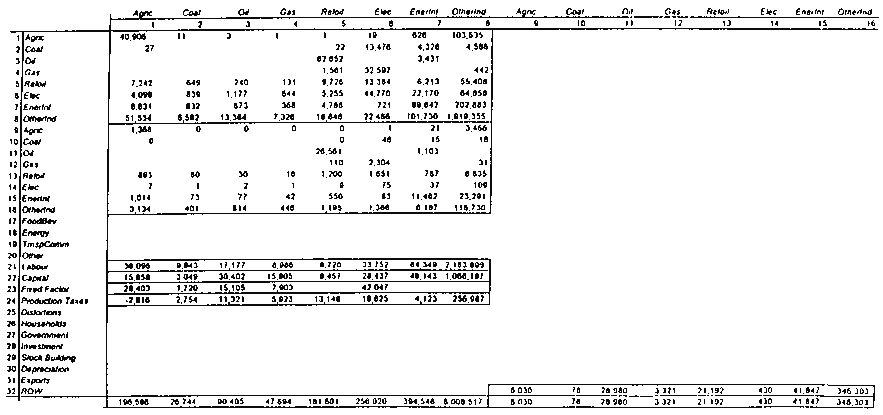
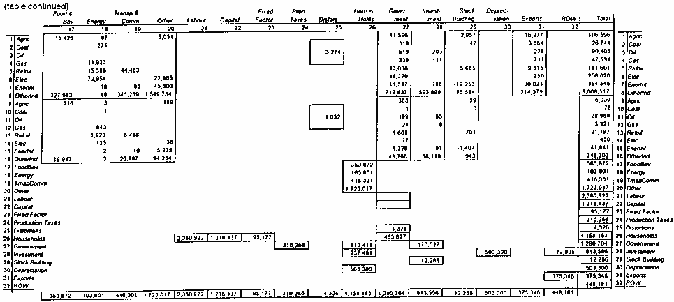
From: OECD (1993b)
The model is myopic. It solves for a sequence of new equilibria for future periods, based on assumptions about exogenous trends in the rate of population and labor productivity growth and technology change, as well as endogenous changes in capital stocks and fixed factor supplies.
2.2 Notation | Contents |
For clarity and consistency in the description of the production structure and other parts of EPPA, the following notation is employed. (A full list of variables and definitions is provided in Appendix 1.) Key indices are:
- I = {i} indexing production sectors;
- R = {r} indexing regions;
- C = {c} indexing consumption sectors and
- T = {t} indexing periods;
- l, k, e, f = indices identifying labor, capital, energy, and fixed factors.
- T = {t} indexing periods;
There are a set of flow aggregates, with precise definitions indicated by the subscripts above:
- Xi,r,t = sectoral gross output;
- Xai,r,t = an Armington output, which is a CES aggregate variable using domestic and imported goods as two arguments;
- Xii,r,t = an imported output within the Armington bundle;
- Xdi,r,t = Domestic output within the Armington bundle; [4]
- Yc,r,t = a consumption good.
- Xii,r,t = an imported output within the Armington bundle;
Then there are the three primary input factors:
- L = labor;
- K = capital;
- FFi = sectoral fixed factor.
- K = capital;
- P = price.
2.3 Production Structure | Contents |
The EPPA model, in a modification of the original GREEN version, permits a choice among ways to represent factor substitutability within production sectors, with either putty-putty, mixed vintage, or fully-vintaged specifications for capital inputs. The "putty" portion of the production structure is a multi-layer CES function calibrated with the 1985 SAM tables for the 12 regions. Eqs. 2.2 to 2.7 are EPPA's CES production functions in the order of top-down nesting, where the rs indicate the CES substitution parameters. The corresponding substitution elasticities are shown in Table A1 of Appendix 2.
[5] The structure is shown in Figure 1.
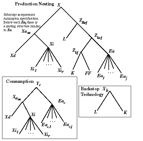
Figure 1. Production Nesting, Backstop Technology, and Consumption.
Eq. 2.1 is the top-layer of the production function. It states that sectoral output X is a linear function of intermediate inputs Xa and an interim quantity variable, Z, comprised of labor, energy, capital and fixed factor,
 [Eq. 2.1]
-
 [Eq. 2.2]
-
 [Eq. 2.3]
-
 [Eq. 2.4]
 [Eq. 2.5]
Eq. 2.1 is the top-layer of the production function. It states that sectoral output X is a linear function of intermediate inputs Xa and an interim quantity variable, Z, comprised of labor, energy, capital and fixed factor,
 [Eq. 2.1]
-
 [Eq. 2.2]
-
 [Eq. 2.3]
-
 [Eq. 2.4]
 [Eq. 2.5]
-
 [Eq. 2.6]
-
 [Eq. 2.7]
Equilibrium factor demands, by sector and region, and prices for factors and sectoral outputs, can be derived in the usual manner from the primary and dual solutions of the cost minimization problem with the above technology.[6]
The three capital vintaging specifications in EPPA differ in the extent to
which the factor proportions can change after the initial investment in a
capital good is made. In all three cases, current technology and input prices
determine the factor proportions of new investment. In the putty-putty case,
there is no distinction between old and new capital: the inherited capital
stock adjusts its factor proportions and technical efficiency to changes in
relative prices and technology as fully as does new capital. By comparison, in
both the vintaged cases, the factor proportions and technical efficiency of the
inherited capital stock are frozen for all periods subsequent to its initial
creation. In effect, each vintage of the surviving capital stock is Leontief,
with technical coefficients determined initially by the CES functions described
above and the input prices and level of technology in the initial period. In
addition to the differing assumptions about the malleability of the inherited
capital stock, the fully vintaged specification makes a different assumption
about the survival of the capital stock. In the mixed vintage specification,
"old" capital is one composite aggregate for which the technical coefficients
are the average of the Leontief coefficients of the constituent vintages
weighted by the depreciated quantity of each vintage. In the fully vintaged
specification, each depreciated vintage is identified separately for five
succeeding periods and then eliminated. As a result of this truncation, the
quantity of "old" capital is somewhat less than in either the putty-putty or
mixed vintage specifications.
Emissions are denoted EE, with the particular gas and sector of origin
indicated by subscript indices. Recall that i indicates a production
sector, e is a subset of i indicating an energy sectors, and that
b is a backstop sector. These sectors are listed in Table 1. To these
we add two new indices:
G = {g}, indexing types of gases, also listed in Table 1, and
S = {s}, indexing subsectors of origin of emissions.
With these definitions we can describe how emissions are calculated. Sample
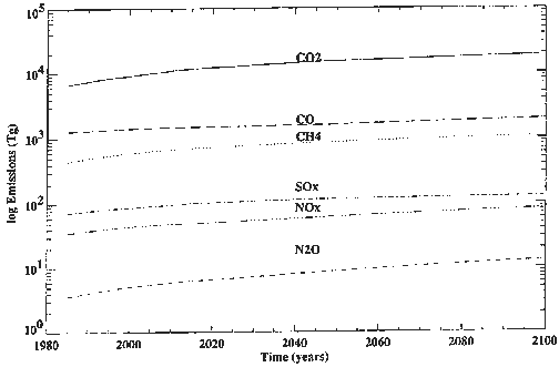
results for CO2 emissions are shown in Figures 2 and 3;
corresponding results for the trace gases are shown in Figure 4.
Carbon Dioxide. Aside from emissions from deforestation, all
CO2 emissions
are ascribed to the region where they are generated. For each region, emissions are
calculated as
Emissions from deforestation are exogenously determined, and are added to the
emissions driven by the activity levels generated by the EPPA model. In the
results shown below, these emissions are assumed constant at estimated 1985
values from 1985 to 2000, and thereafter to decline linearly to zero in 2050.
Methane. Total methane emissions are the sum of the emissions from a
number of sources. First are emissions from agricultural activities, which are
driven by activities in the aggregate agricultural sector:
Nitrous Oxide. Emissions of N2O result from a number of agricultural, industrial, and energy-sector activities, and from biomass burning (this last source also treated separately below). The estimates of emissions from fertilizer use and nitric acid production are of the form of Eq. 2.10, with appropriate values of ag,s. Adipic acid production is the same, only related to the Xdi for i = Other Industries and Services. Emissions from fossil fuel combustion takes the form of Eq. 2.11 for e = refined oil, with an appropriate value of ag,e applied. Emissions from the extension of cultivated land are based on a simple growth rate applied to emissions as estimated in 1985. Parameter values are given in Table A4 of Appendix 2.
Nitrogen Oxides. The main anthropogenic source of NOx is fossil fuel combustion from stationary and mobile sources, with additional emissions from petroleum refining, cement manufacture, nitric acid production, and biomass burning. At present, the prediction of NOx emissions from all sources but biomass burning is modeled by an equation of the form of Eq. 2.10, with Xdi from Energy Intensive Industries, and appropriate values of ag,s.
Chloroflurocarbons. Chloroflurocarbons are assumed to follow the phase-out schedule of the London Amendments to the Montreal Protocol.
Carbon Monoxide and Sulfur Oxides. Anthropogenic sources of CO include fossil fuel combustion, the production of steel, pig iron, and ammonia, and the burning of refuse and agricultural waste, sewage, and biomass. The sources of SOx include coal and petroleum use, smelting of non-ferrous ores, production of sulfuric acid, pulp and paper, incineration of wastes, and biomass burning. (As with other gases, emissions from biomass burning are treated separately.) For each region, emissions of these two gases are modeled by two equations each, one representing energy use and the other covering industrial activity.
For CO, the emissions from fossil fuel use are projected as resulting from the use of coal and refined oil:
2.4 The Demand for Crude Oil and Natural Gas | Contents |
The demand for crude oil and natural gas differ from the demand for
other energy inputs and intermediate inputs in that, for each, domestic
production and imports are perfect substitutes. Furthermore, each is traded
inter-regionally with perfect substitutability, as Heckscher-Ohlin goods,
instead of as Armington goods. Within each region, therefore, the production
sectors--as well as the consumption sectors, government, and investment--treat
crude oil and natural gas from domestic output and from imports as the same
good. It is assumed that trade barriers for oil and natural gas are
non-existent, except for taxes or subsidies that may cause the domestic prices
for these two goods to differ among regions. Instead of the usual definition
for Armington goods (Eqs. 2.6 and 2.7), the aggregate demand for oil and
gas takes the following form:
Equivalently, we can assume that for oil and gas ra1 = +1.0 and ra2 = +1.0 in Eqs. 2.6 and 2.7.
 [Eq. 2.8]
2.5 Emissions of Greenhouse-Relevant Gases
Estimates of emissions of greenhouse gases, and other gases which
produce scattering aerosols or otherwise influence the atmospheric chemistry,
are driven by various activity levels within the model. With the exception of
emissions from deforestation and some components of biomass burning,
CO2 emissions are calculated directly from the period-to-period
levels of energy sector activities. The prediction of trace gases begins with
base-level emissions in 1985, and the emissions in subsequent periods are
related to changing levels of energy and non-energy activities using elasticity
factors, as detailed by Liu et al. (1996).
where
 [Eq.2.9]
The first term in the expression is the emissions at the point of consumption,
where Xa is the Armington aggregate of energy type e, TJ85
is the coefficient converting the dollar value of energy of type e,
expressed in millions of 1985 U.S. dollars, into heat units (exajoules), and
is the coefficient converting heat units into CO2
emissions. The values of TJ85 and are provided in Tables A2
and A3 of Appendix 2. The second term in Eq. 2.9 is the emissions at the
point of production of the carbon liquids backstop, which is available in only
the USA, the Other OECD (representing Canadian and Australian resources) and
the Energy Exporting LDCs (representing Venezuela among others). (The backstop
technologies are described in Section 3.5.) This technology is assumed to
produce refined oil after extensive processing, and the release of
CO2 at the point of production is expressed as a fraction, l,
of the CO2 emitted by the corresponding refined oil at the point of
consumption. In the sample calculations shown below, l is set at 0.8.
where s = rice paddies, enteric fermentation and animal waste, and Xdi is production in agriculture. Components of energy sector methane are estimated as
 i = agriculture, [Eq. 2.10]
Landfills and domestic sewage are modeled in the same fashion, with landfill emissions driven by per-capita GDP and emissions from domestic sewage related to population itself. Methane also is emitted from biomass burning, which is covered below.
 e = coal, natural gas. [Eq. 2.11]
where e1 denotes coal and e2 is refined oil, and lg is 0.2. Emissions from industrial sources are modeled as  [Eq. 2.12]
where Xdi is the activity level of energy-intensive industries. For SOx the equations are the same, with lg set to 0.66 and appropriate values of the elasticity, as described in Table A4 of Appendix 2.
 [Eq 2.13]
Biomass Burning. Biomass burning encompasses a variety of activities, which can be roughly classified into the five categories: (1) the burning of the world's forests for land clearing and agricultural use (including both shifting agriculture and permanent agriculture), (2) the annual burning of savannas to control pests, weeds, and brush accumulation, (3) prescribed burning in temperate and boreal forests, (4) the annual burning of agricultural stubble and waste after harvest, and (5) the burning of wood for energy production. These processes emit CO2 and the trace gases CH4, N2O, NOx, SOx, and CO.
In the case of CO2, annual burning of savannas, brushland, and agricultural wastes does not contribute net emissions into the atmosphere, since the CO2 released is re-absorbed by re-growth the following year. Only deforestation with burning of the wood represents a significant net CO2 emission into the atmosphere, as long-term stores of carbon are released with no possibility for re-absorption in the short term. For all other greenhouse-relevant gases, however, all biomass burning yields net releases since they are not re-absorbed by plant growth. With the exception of prescribed fires in temperate forests, biomass burning takes place almost exclusively in the tropical and subtropical regions of the world. Since EPPA does not aggregate into tropical and other regions, we compute emissions from biomass burning as a global value. Agricultural sources of trace gases (category 4 above) are estimated using a relation of the form of Eq. 2.10, with Xdi from aggregated global agriculture, and appropriate values of ag,s. Other sources (categories 1, 2, 3 and 5 above) are assumed to follow the same pattern as the exogenous assumption for CO2 from deforestation.
Annual burning of savannas for control of pests and brush accumulation, prescribed forest fires, and burning due to shifting agriculture is treated as constant over time at their 1985 levels. Shifting agriculture is not expected to grow much, but permanent conversion of forests to land for agriculture or pasture is growing. The harvesting of wood for energy also contributes to deforestation. Emissions from permanent deforestation and fuelwood harvesting grow at the rate of deforestation, which is exogenous as noted above. Burning of agricultural wastes is assumed to increase as agricultural production increases, and is modeled by a relation like Eq. 2.10, with appropriate parameters.
Distribution by Latitude. Emissions of all gases are needed by 7.8 degree latitude band, for inclusion in the MIT coupled chemistry-climate model, because the atmospheric chemistry is influenced by the geographical distribution of emissions as well as their global amount. Global emissions of the long-lived gases (CO2, N2O, CH4 and the CFCs) are distributed by a function that remains constant over time. Emissions of the short-lived gases (CO, NOx, SOx) are distributed within each region according to population distribution, and the latitudinal totals are simply the sum of the 12 regions. Thus with differential growth and emissions among the 12 regions, the latitudinal distribution shifts over time.
The demand for production goods by the investment sector is defined in the
same manner as for consumption:
Government expenditure includes two parts. One is for the direct transfers to
the consumer; another is expenditure for inputs required for the production of
government services. Government revenue comes from taxes on household and
production sectors. The difference between government expenditure and revenue
is government savings (Sg). The production function of the
government good takes the following form:
Initial current account imbalances among the regions are phased out over time.
The absolute values of the imbalances decline gradually during the first four
periods, and are eliminated completely in the fifth period. Initial inventory
and exogenous investment (i.e., the differences between total investment and
household saving in the SAMs) are treated in a similar way. They are reduced
gradually in the first four periods, and disappear completely in the fifth
period.
Finally, based on the above closure rules, the EPPA model solves for an
overall equilibrium in which the following market clearance conditions are
met:
Labor productivity improvement in region r is expressed as an index
over time. It is assumed that all regions start with relatively high, though
different, labor productivity growth rates, but converge to some common, lower
annual labor productivity growth rate by the year 2100. In the reference runs
shown below, this target is 1.0% for OECD regions (USA, JPN, EEC and OOE) and
EEX. All other regions converge to 2.0% per annum by the year 2100. Based on
the above assumption, Lpr(t), the labor productivity
level, is:
Finally, Lr(t), total labor supply is defined as:
2.6 Consumption, Investment and Government Expenditure
Each region has a representative consumer who maximizes a utility
function in consumption Yc and a minimum consumption level,
qc:
subject to the budget constraint on disposable income Id. Disposable
income is defined as the sum of returns to all primary factors, plus government
transfers (Gtr), minus savings (Sh) and
household taxes (Th). Namely, [Eq. 2.14]
where Ls, Ks, and
FFs are total regional supplies of labor
(specified in efficiency units as described in Section 3.1) capital and fixed
factor, respectively, and  [Eq. 2.15]
On the supply side, consumer goods are produced using inputs from the three
non-energy production sectors plus energy inputs for two of the consumer goods,
fuel and power and transport and communication.
where the energy inputs are CES aggregates of the various energy sectors: [Eq. 2.16]
As with the production sectors, the prices of consumer goods, and consumer
demand functions for those goods, can be derived from the corresponding optimization problem. [Eq. 2.17]
where
 [Eq. 2.18]
Note that investment, like consumption, does not require direct primary factor inputs. [Eq. 2.19]
where
 [Eq. 2.20]
Finally, in the EPPA model, stock-building entries in the 1985 SAM tables are
treated as residuals that are added to or subtracted from the endowment of the
consumer. Therefore, no stock building relationships are specified.
 [Eq. 2.21]
2.7 Closure Rules and Market-Clearing Conditions | Contents |
The levels of government expenditures, both production and transfers,
are exogenous. The tax revenues, both from household taxes and from indirect
taxes on production, are also exogenous. For each region, both expenditure and
revenue are set as a fixed share of total GNP. These assumptions imply that
the initial government deficits or surpluses remain fixed at the initial (1985)
share of GNP.
where EXi = exported output. Equations 2.22, 2.23 and 2.24
are clearing conditions for primary factor markets. Equation 2.25 is a
commodity market clearing condition. It states that the production of sectoral
output is equal to domestically produced intermediate goods demanded by other
sectors plus domestically produced "final goods" including exports.
 [Eq. 2.22]
 [Eq. 2.23]
 [Eq. 2.24]
 [Eq. 2.25]
3. Assumptions About Growth and Technical Change | Contents |
3.1 Labor Supply
The exogenous rates of population growth in different regions over the next
century are based on United Nations' estimates (Bulatao et al., 1990).
In general, the UN estimates anticipate moderate population growth in developed
countries and rapid population growth in developing countries in the near
future. The population growth rates in both regions slow down over time.
Based on United Nations estimates, we calibrated Popr
(t), the population growth trend in region r, to fit the
following formula:
The coefficients, ginfinity and g1 are the ratios
of asymptotic level and the second period level of population relative to the
base year, respectively. The initial population and coefficient values are
given in Tables A2, A3 and A4 in Appendix 2. [Eq. 3.1]
 [Eq. 3.2]
Here g0 is the initial labor productivity growth rate;
gn is the terminal labor productivity growth rate (set at 1%
or 2% in the runs below); Hoz is the time horizon of the model and is
115 years (from 1985 to 2100). The values of g0 are given in
Table A8 of Appendix 2. [Eq. 3.3]
 [Eq. 3.4]
 [Eq. 3.5]
 3.2 Capital Formation | Contents |
In the EPPA model, the mechanism of capital formation has been changed
significantly from that in GREEN. The capital supply in region r at
period t, K(t), is given by the following relationships:
where Sh,r is household saving, Yr is GDP;[7] rr is the
return to capital; wr is the wage rate;
r is the benchmark capital depreciation rate derived from the
SAM table; sr is the initial saving share and s is a damping factor. In the actual programming, the time differences are compounded
for each five year step based on annual data. Several small adjustments which
are made to insure that initial inventory and trade imbalances are properly
incorporated into the S = I identity are not shown in equations
3.6 and 3.7. These imbalances and the corresponding adjustments are zeroed out
by the fourth period. [Eq. 3.6]
 [Eq. 3.7]
The treatment of capital formation in EPPA brings neoclassical investment
theory into the empirical CGE model environment by making savings a function of
the shadow price of capital.[8] This is in
contrast to GREEN, which adopts a balanced growth assumption, determines
savings exogenously, and adjusts capital productivity (usually negatively) to
maintain balanced growth on a pre-determined growth path. In the EPPA model,
household savings adjust according to the relative scarcity of capital in the
economy. Both r and w are set to 1.0 in the base year.
Therefore, if r/w is subsequently greater than one, capital is in
short supply, relative to the labor supply in efficiency units, and vice versa.
In response to the short supply of capital, household savings are increased as
a share of total GDP. Because r/w deviates significantly from
1.0 in a few initial periods, a damping factor is applied to reduce the
fluctuation in saving levels. The damping factor in equation 3.7 is
set at 0.25 in the current version of the model; and the values of
sr are given in Table A9 of Appendix 2.
Within the time horizon of the model, the potential supplies of fixed factors
in agriculture, coal and electricity are assumed to have no upper bound. The
actual supplies in these sectors are functions of their own prices and previous
period's supply level. In fact, FFi,r(t), the fixed
factor supply of sector i, region r and period t, is:
Fixed factor supplies in the oil and gas sectors are exhaustible within the
time horizon of the model. In these sectors, the fixed factor supply is
proportional to the sectoral and regional resource depletion profiles which are
functions of discovered and yet-to-find reserves, an exogenously specified
depletion rate and output prices. The determination of resource depletion
profiles for oil and gas in the EPPA model is similar to that in GREEN.[9]
In order to reflect the parallel effect of technological progress on the
supply of oil and natural gas, it is also assumed that the fixed factor input
requirements for oil and natural gas are reduced over time. The fixed factor
improvement rate is set at 1% per year for all regions.
Backstop technologies in the EPPA model have linear production structures with
two inputs, labor and capital, which reflect the assumed infinitely
reproducible nature of this output. Thus, we have:
In the EPPA model, backstop technologies are introduced when
The main advantage of programming in MPSGE/GAMS is that the solution algorithm
and the economic model can be separated. This separation makes it possible for
users to make changes in model structure, and to introduce new assumptions,
without extensive re-programming and debugging. A professional division of
labor is allowed, in which the implementation of a robust solution algorithm
for CGE models is left to mathematicians and computer scientists, so the
modelers can focus on the economic structure of the model.
In the EPPA model, any single solution consists of one assumed equilibrium
imposed on the benchmark data for the base year, 1985, and 23 calculated
equilibria for five-year intervals through 2100. Each new equilibrium of
supply, demand and relative prices is calculated based on exogenous changes in
population, labor productivity and the AEEI rate and endogenous changes in
saving levels and fixed factor availability. Since the model is myopic, no
consideration is given to potential changes in future prices or resource
availability in determining each period's equilibrium.
When CO2 reduction policies are imposed, the EPPA model generates a
set of new sequential equilibria that are consistent with policy constraints.
An entire path with 24 periods generated from policy shocks is a
"counter-factual" scenario relative to baseline path.
Both energy taxes and carbon quotas depress the demand for output from the
energy sectors. The revenues from taxes and quota allowances are assumed to be
transferred to the representative consumer as a lump sum. Since the taxes or
quotas distort the equilibria in the economy from the no-policy baseline, the
imposition of these policy instruments often reduces GDP. It is possible,
however, for regional GDP to increase when the tax or quota has the effect of
off-setting the distortion from an existing subsidy. In all the solutions the
conventional assumption of CGE modeling is maintained that all productive
resources are always fully employed.
In policy comparisons, GDP is often used as an approximate measure of general
welfare, and a change in GDP is interpreted as a measure of resources foregone
as a result of the policy constraint.[13] In
EPPA, we do not use real GDP, strictly defined, as our measure of welfare, but
rather real household consumption. We do this to avoid problems involved in
the definition of real GDP in this type of model, and the response of this
variable to policy perturbations. Real GDP is defined on the input side as the
inner product of primary factor prices and quantities. When perturbed by
policy, factor quantities adjust very little because factors are fully
employed. Therefore, typically real GDP changes little. Household consumption
provides a more accurate reflection of welfare. Since consumption consists of
four goods in EPPA, we are able to capture the differential effects of policy
measures on the composition of household expenditure (for instance, between
energy and non-energy intensive goods) as determined by our specification of
consumer utility.
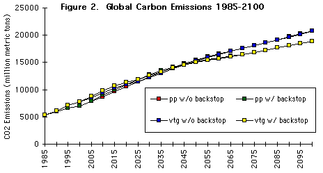
Figure 2. Global Carbon Emissions 1985-2100.
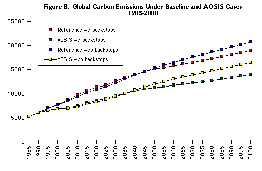
As can be seen in Figure 2, the fixity of capital does not matter in the long
term because the vintage specification reverts to putty-putty in 2040. The
assumptions about backstop technologies do make a discernable difference,
however. Given the assumptions incorporated in this EPPA run, the net effect
of introducing both carbon-intensive and carbon-free backstop technology is a
lower carbon trajectory over the latter half of the 21st century.
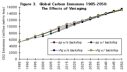
The nearer-term effect of the different assumptions about capital fixity is
shown by Figure 3, which is an enlargement of Figure 2 for the years 1985-2050.
Since there is an assumed tendency toward improved energy efficiency and higher
energy prices over time, successive vintages of capital are less energy and
carbon-intensive. Global emissions are higher when the energy efficiency of
the older vintages is assumed fixed, but by 2025 the initial capital stock has
been completely replaced and it is only new technology that matters.
Figure 3. Global Carbon Emissions 1985-2050: The Effects of Vintaging
Figure 4. Global Emissions of CO2 and Trace Gases
In our reference predictions, the paths of emissions with and without the
backstop technologies cross over in the 2040s. Initially, the projections of
carbon emissions, when backstop technologies are available, are higher than
projections without backstop technologies, because the carbon backstop is used
earlier than the carbon-free backstop. However, as the carbon-free backstop is
deployed, the emissions path for the backstop scenario turns lower by 2050 and
is progressively lower as seen in Figure 2.
The main cause of the projected overall increase in global CO2
emissions is growth in regional GDP as shown in Table 3[14], which shows 1985 GDP, average annual rates of growth in
subsequent intervals, and 2100 GDP as a multiple of 1985 GDP. The last column
shows that regional differences in GDP growth are considerable. With the
exception of Japan, the GDP for the OECD regions (the first four rows)
increases about five-fold, while regions such as China, India and the Dynamic
Asian Economies increase by multiples of 20 to 25 by the year 2100. The
differences reflect the effect of assumptions concerning population growth and
increases in labor productivity, as well as differences in capital formation.
TABLE 3. Changes in regional GDP.
3.3 Fixed Factor Supply | Contents |
Five of the eight production sectors require fixed factor inputs.
These five sectors and their fixed factors are Agriculture and land, Coal and
coal reserves, Crude Oil and Natural Gas and their reserves, which are
depletable, and Electricity, Gas and Water Distribution for which hydro and
nuclear power capacity are represented as fixed factor endowments. The units
of fixed factor supply are in 1985 US dollars and are measured as fixed factor remunerations.
Here pf is the fixed factor price, pu is the price of consumer's
utility and sf is price elasticity of fixed factor supply. [Eq. 3.8]
 3.4 Energy and Fixed Factor Productivity Improvement | Contents |
The EPPA model introduces productivity improvements in the input
requirements for energy in the non-energy sectors and for the fixed factors in
oil and natural gas, similar to that described above for labor. Like GREEN,
EPPA adopts an assumption of autonomous energy efficiency improvement (AEEI) to
reflect the observed long-run historical trend of reduced energy requirement
per unit of output. For three non-energy production sectors, four consumption
sectors, government and investment sectors, the input energy bundles have the
following feature to reflect the AEEI:
where Ee is effective energy input in sector i; ge is AEEI rate. In the current EPPA reference,
ge is set at an annual rate of 0.0075 for all sectors and across all regions. [Eq. 3.9]
3.5 Backstop Technologies | Contents |
The EPPA model allows for the introduction of backstop technologies
which produce perfect substitutes for conventional energy. In Version 1.6 of
this model, two backstop technologies are implemented: (1) a carbon-free
electricity production backstop, representing opportunities such as solar or
advanced nuclear technology, and (2) a relatively carbon-intensive substitute
for refined oil, based on world resources of heavy oils, tar sands and oil
shale. This carbon backstop emits CO2 in the production process of
the fuel, as well as from the consumption of the final product, refined oil.
The carbon-free electric backstop is assumed to be available to all regions.
The carbon backstop is assumed producible only in USA, OOE, and EEX, which have
large reserves of oil shale and tar sands. The liquid fuel output is traded
internationally as refined oil (an Armington good).
and
 [Eq. 3.10]
where, subscript b represents backstop production, subscript c
represents conventional production; and a and b are the Leontief coefficients. The initial period or benchmark unit cost of the backstop technology, cb,i is the sum of the Leontief
coefficients. By definition, the backstop technologies are not economic in the
initial period, and thus the sum of these coefficients is greater than 1.0,
which is the initial price of the conventional fuel for which the backstop can
substitute.[10] The values of
cb,i are in Table 10 of Appendix 2. [Eq. 3.11]
 [Eq. 3.12]
Of course, by the Kuhn-Tucker theorem, in the final equilibrium:
 [Eq. 3.13]
In the model, we also restrict the entry of backstop technology to occur no earlier than the year 2000.
 [Eq. 3.14]
4. The Solution Concept | Contents |
4.1 Algorithm
The EPPA model is programmed in GAMS language (Brooke et al.,
1992). Under the GAMS platform, the static structure of the EPPA model is
written in MPSGE (Rutherford, 1994), which is an abstract, high-level language
for formulating CGE models. The equilibrium prices and quantities of the EPPA
model are solved by using the PATH solver, a generic algorithm for solving MCP
(Mixed Complementary Programming) problems.[11]4.2 Sequential Equilibria | Contents |
Most CGE models are static models. Benchmark data are calibrated to
fit the designed economic structure, and an equilibrium solution is obtained.
Then "counter-factual" scenarios are imposed on the model to explore the
impacts of potential policies or shocks. The EPPA model operates in this
manner.5. Policy Instruments | Contents |
Policies implemented in the EPPA model may take the form of either
price instruments (taxes or subsidies) or quantitative instruments (quotas).
The price instruments that have, so far, been specified are ad valorem
energy taxes levied on unit[12] energy
consumption or, ad valorem carbon taxes levied on units of carbon
content in energy output. The quantitative instruments are CO2
emission quotas imposed on individual regions or block of regions or all
regions. When imposed globally or on a block of regions, quotas can be
tradable among regions.6. Sample Results | Contents |
In order to illustrate the behavior of the EPPA model, we provide some
simulation results based on the parametric values and other assumptions
described above. In Section 6.1 we show various features of the model in
typical reference run that is unconstrained by policy relative to GHGs.
Section 6.2 presents the results of imposing a sample policy prescription.
6.1 Reference Run | Contents |
Figures 2, 3 and 4 present the basic output of the EPPA model, which is
the time path of global emissions of CO2 and other gases from 1985
through the year 2100. In Figure 2, four cases are presented for
CO2 emissions, in which the effect of two of the improvements
incorporated in EPPA are shown, namely, varying assumptions about the presence
of backstop technology and the treatment of capital. The closed symbols in
Figure 2 represent projections in which the backstop technology is assumed not
to be available, and the open symbols denote the presence of backstop
technology. Similarly, squares represent the putty-putty assumption of
completely flexible capital, and the diamonds denote the fully vintaged
specification of the capital stock. The mixed vintage capital specification is
not illustrated here. (The emissions of trace gases, in Figure 4, are for the
case with backstops and full vintaging.)