|
Figure 1: The second-order system, amplifier (bottom left)
and breadboard (top)
|
|

|
Figure 2: Drawing of the second-order system used in this lab
|
|
In this lab, students examine the effects of feedback control on the second-order plant of labs 3 and 4 (figure 1 and 2). The controller consists of an op-amp circuit that adds both proportional and derivative control. Proportional control enables the stiffness to be increased (faster rise time), but the damping ratio to be decreased. The larger overshoot and settling time caused by this lower damping ratio is reduced by derivative control. Derivative control (along with proportional control) enables the damping ratio to be increased.
|

|
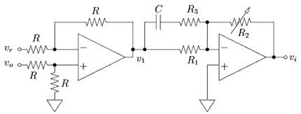
Figure 3: Op-amp circuit for implementation of proportional and lead
control with an adjustable gain
|
|

|
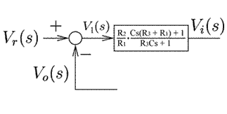
Figure 4: Block diagram equivalent of figure 3
|
|
In figure 3, the op-amp circuit of this lab is shown. This circuit allows us to implement proportional and lead control with an adjustable gain. The left op-amp is used to create the summation point. The inputs of the first op-amp are switched compared to its equivalent block diagram in figure 4 to compensate for the second inverting op-amp. Students can compare this PD-control with proportional control by leaving the capacitor and R3 out.
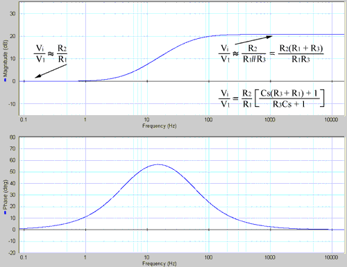
Figure 5 shows the bode plot of this controller. The values of the resistors and capacitor are:
R1 = 68    kΩ
R2 = 68    kΩ (1 MΩ potentiometer in figure 5 used to create unity gain at low frequencies)
R3 =  6.8  kΩ
C  =  0.47 μF
Figure 5 shows the approximations for lower and higher frequencies. Below the break frequency 1/C(R1+R3) the system's transfer function approaches R2/R1. Above the second break frequency 1/R3 the system's transfer function approaches R2/R1//R3 =
R2(R1+R3)/R1R3.
|

|
Figure 5: Bode plot of the controller used in this lab, with approximations for lower and
higher frequencies
|
|
Students can adjust the potentiometer to obtain different rise times with both the P-controller and the PD-controller. They can estimate the position of the poles at each setting, thus creating root-locus plots. Finally, the students can compare the plot of the proportional controlled system with the PD-controlled system.
|
The examples of prelab and lab assignments given below come from
Fall 2002, when this project was "Lab 8".
prelab9_2002f.pdf
lab9_2002f.pdf
|