EGS MODELING for WINDOWS
EGS Modeling for Windows is a tool for economic analysis of geothermal systems. The software was developed by the MIT Energy Laboratory as part of its research into EGS systems sponsored by the Geothermal Technologies Office of the U.S. Department of Energy. The program can run in a simulation mode or can optimize the parameters specified by the user. The program starts with a customizable default input and the user is able to edit the values of the input parameters. The user can run the model and generate different reports which can be saved, printed or viewed at the user’s convenience. All these features are driven by a windows style graphical interface and are easily accessed by the intuitive interface elements of the software.
This file is divided into following sections:
The Model
To install EGS Modeling for Windows:
1. Run install.exe which should be in your distribution package
2. Follow the instructions given in the series of dialog boxes in the setup program. After you answer all of the questions, the installation program will take about four minutes for completing installation.
For more details see Installing EGS Modeling for Windows
To run EGS Modeling for Windows:
1. Start Microsoft Windows NT or Windows 95.
2. From the Start menu select Programs.
3. Select EGS Modeling for Windows to open the application.
4. From the File menu, select New to start a new run.
5. From the Input menu, select Start to display the input forms.
6. Cycle through all the dialog boxes using the Next or Previous buttons and edit the values of the parameters in each form.
7. Click OK when you are satisfied with all the parameter values you have entered.
8. From the File menu, select Save to save your case.
9. From the Run menu, select Run to run the model
10. From the Results Menu, select the report of interested to view. You can cycle through different reports by using the Next or Previous buttons.
For more details see Inputting the Parameters, Running the Model, Browsing the Reports, Managing your Files, Setting the Default Values.
EGS Modeling for Windows is written in Visual Basic 6.0. Even if the interface components are not resource hungry, being a visual basic application following requirements should be met:
Installing EGS Modeling for Windows
Once you get the distribution file, save it to a folder. Then double click on the icon that says install. The EGS software is distributed in a self-extracting installer format, so it will first uncompress itself then start the installation procedure. During the installation, you will be asked to specify the directory where you want to install the program. The total installation might take around 5 minutes.
During the course of installation, if the installation program determines that your system does not have updated Visual Basic runtime files, it will install those files and ask you to reboot the system. If this happens, you have to restart the installation process once the system reboot is over.
Installer might also complain that the setup program is trying to copy a file that is older than the one already installed in the system. The installer might report this problem even if you are installing the EGS software for the first time. Click on "No to All" to resume the installation.
Installer will create a program pointer in the Start/Programs menu with the name EGS Modeling for Windows.
If you want to override previous installation of EGS software, you can either specify the same folder as before or you can specify a new folder. Even if you specify the folder that has previous version of EGS software, installer will not delete the data and report files that you created.
Note: If you are running Windows NT, unless you are logged on as an administrator, you might have to rename install.exe to something else before you can run the installer.
Inputting the Parameters
When you open the application, a main window with a menu bar will appear on your windows desktop. In order to create a case, select Start from the Input menu. You will then be prompted with the Engineering Parameters dialog box. As you will realize, the dialog box comes preloaded with software default values. Now you can change the values of the parameters as you wish. Cycle through the different input forms using the Next or Previous buttons and enter your values.
These are the different types of input components that you might encounter spread across different dialog boxes:
Edit Boxes: Edit boxes are text input areas where you can click and input the numbers directly. When a particular input is not required by the model then the edit boxes related to the input are disabled. When disabled, the text appears grayed.
Drop-Down Lists: A Drop-down list is a control window that contains a list of items that can be selected by the user. Click on the drop-down arrow to display the list. In order to select the item you are interested in you can click on the list and scroll up or down as you like and click on the item you want to select
Radio buttons and Check boxes: Radio buttons look like a white circle on the form where you can click and make a small black dot appear in the center and thus select the option. Check boxes are squares and will have a X on it when selected. You can make only one selection in a radio box while you can make as many selections as you want if check boxes are used.
The interface is driven with a lot of validation code that will prevent you from making erroneous inputs. Whenever you make invalid input, you will be asked to edit that value when you try to confirm all the changes that you have made in that form by pressing the OK, NEXT or PREVIOUS buttons. You will also be informed on valid range for the parameter that you are trying to edit. You have to have correct values for all the parameters listed in a dialog box in order to proceed to another dialog box or to confirm the values. If you want to restore to the original values that were there before editing, you can always hit CANCEL and escape out of that dialog box.
The dialog boxes are setup to appear in a sequence with the Engineering Parameters form followed by the Resource Characterization form, Reservoir Model form, Economic Parameters form, Capital Costs form, Operation and Maintenance Costs form and Optimization Parameters form in this particular order. You can go from one form to another by simply pressing NEXT button in each dialog box or if you want to follow the form sequence in the opposite direction you can use PREVIOUS button.
Parameters set in some of the dialog boxes will affect what is going to appear in some other dialog boxes. As a consequence, some of the input fields might appear disabled and grayed out in some dialog boxes. Studying the description of each parameter and their dependency in the EGS model should be helpful in determining the cause for any such effect seen in some of the form parameters. For instance, setting the Mode of Operation to Simulation in Engineering Parameters form will inactivate all the input parameters in Optimization form.
Individual parameter forms can also be accessed directly from the menu instead of having to cycle through the whole sequence. All the forms are listed under Input menu. Individual forms can be selected from the menu and activated. The forms are setup to be modal forms so activating more than one form at the same time is not allowed by the system. Whenever there is an active form, the menu bar is disabled and thus will restrict from having multiple forms.
When you are done changing all the system parameters, you can hit OK and that will take you to the top level window.
Running the model
In order to run the model, select the Run menu and click on Run. This will start the simulation or optimization process which takes around 15 seconds to complete. While the code is running a wait message appears on the screen. When it is done, the program will display a message saying "Simulation completed successfully" or "Optimization completed successfully".
If you are running the model on the current data set for the first time, first you will be asked to save the current data set, only then you may proceed to Run -> Run to run the calculation.
Browsing the reports
The Report generated by the program is modular and each module can be accessed separately from the Reports menu. Selecting the appropriate report module under the Reports menu will bring up the desired report module. Like input forms, report forms are also arranged in a sequence. So pressing the PREVIOUS or NEXT buttons will bring up the previous or next module in this sequence: Full Reports, Summary Results, Economic Parameters, Engineering Results, Resource Characteristics, Reservoir Parameters, Capital Costs, Operation and Maintenance Results, Power Generation Profile and Heat Extraction Profile.
In the Power Generation Profile report and Heat Extraction Profile report, each column when clicked will bring up a graph window that will plot the parameter selected against the time in years. Just hit DONE on graph dialog to return to the profile. All the parameter listed in the profile can be plotted against time with this procedure.
Individual graphs can be accessed from the Graphs menu and the appropriate category. The graphs provided by the program are divided into two categories:
Thermal Drawdown, Geofluid Temperature, Pump Power, Net Power, First Law Efficiency.
ThermoPower, Heat Extracted, Reservoir Heat Content, Percentage of Total Heat Mined.
If these graphs don’t meet your requirements, then you can copy the data to the windows clipboard and paste them in Windows Excel or any other application to do sophisticated graphing or further data analysis. In order to do so, from the Results menu select the Power Generation Profile or the Heat Extraction Profile and click the Copy button. Switch to the application where you want to export the data to and use the paste command for that application (usually Ctrl-V).
The software comes with a facility to print the full report text, Power Generation Profile and Heat Extraction Profile. Pressing Print button on a report form will print the current report module to a default printer set by the windows operating system. The EGS software does not ask for any confirmation or does not let you choose between printers so if the report needs to be printed to a non-default printer then that printer has to be first set as a default printer. In order to do that, go to the windows control panel. Double click on the printers icon. Do a right click on the printer that you want to print to and select Set As Default. Now whenever you issue the print command from within the program, the report will get printed to the printer that you set as default.
Uninstalling EGS Modeling for Windows
To remove EGS Modeling for Windows, do the following:
1. Click the Start Menu.
2. Move the pointer to Settings, then click on Control Panel.
3. Double-click on Add/Remove Programs.
4. Click EGS Modeling for Windows within the displayed list of applications.
5. Click the Add/Remove button.
This procedure removes files installed during the previous EGS Modeling for Windows installation. This Add/Remove Programs procedure, only removes files created by the EGS Modeling for Windows installation program that are used only by EGS Modeling for Windows. Even after you uninstall the software, all the files that you saved in the program’s folder will be preserved.
Managing your files
The EGS program saves two files for each case. The first one is the input file, which stores all the values of the parameters you set in your case. The default extension for the input file is EGS. The second file is the report text file which has an extension rep by default. When the Save As option from the File menu, the system saves the current parameter values in the input file which will have the name that you specify in the File Save As dialog box. It will also store the latest report generated under the same name with rep extension in the same folder as the input file. Thus, if you want to move your files to a different directory, be sure to copy both the files associated with each case.
In the even that the program cannot find the report file for an input file, the program will issue a warning message and prompt you to run the model before you request any reports. In that case the system will not display any report unless you run the model.
The EGS program requires that a case have a name before you can run the model. So if you select Run, from the Run menu after working on a new input file without saving it, the system will ask you to save the case first then proceed to the calculation.
If you want to specify a new file, use File -> Save As or if you want to use the current name you can just use File -> Save option.
It is possible to make your own default value settings for each of the parameters in the system. In order to do so, select New from the File menu, or click on the Start icon on the toolbar. Change the parameter values in the forms as if you were editing a normal case. When you are done changing the parameters, instead of selecting File->Save select File->Save as Default. The software will then store the current case as a template case.
From that time on, whenever you start the software it will load those values set as default. If you reset a case by selecting File -> New or Load Default Values, the same default parameter set will replace the current case.
Status bar
The status bar on the bottom always displays the current status of the program, the name of the current case the user is working on, current time and date.
Toolbar
The toolbar gives the user a quick and easy way to access the tools the user needs to complete a task. To use the toolbar just click a button on the toolbar. The user must use a mouse to select buttons on the toolbar. The user cannot use the keyboard. The EGS Modeling for Windows has the following buttons for quick access to frequently used features:
To create a new case click on ![]()
To open an existing case click on ![]()
To save a case click on ![]()
To edit the input parameters click on ![]()
To run a case click on ![]()
To browse the results click on ![]()
To print the full report click on ![]()
To browse the graphs click on ![]()
To open the help file click on ![]()
Using Help
EGS software has context sensitive help. If you are not sure about some form parameters, click on button that says Help and it will popup help window with description of parameters presented in the dialog box.
If you are looking for some reference, you can browse the help system by selecting content option presented under Help menu. Or if you want to do text search, select search the index under help menu.
EGS Model
The EGS Model is a generalized multi-parameter economic model for optimizing the design and performance of EGS geothermal systems and predicting the break-even price of EGS generated electricity.
Important parameters include:
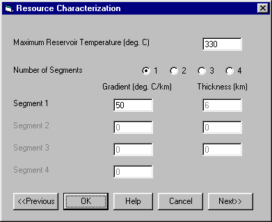
This menu allows configuration of the parameters relating to the geology of the site. The maximum reservoir temperature refers to the maximum attainable temperature that the drilling equipment, casing, etc. can withstand. This temperature limit cannot be violated. The temperature gradient can be given as a single (average) number or break up to four segments. The program assumes a linear increase of temperature with depth. Once an average gradient has been applied by the user, the EGS Model checks to see if the product of the well depth (as indicated by the user in the engineering parameters form) times the temperature gradient plus 15 degrees Celsius (assumed surface temperature) gives a bottom-hole temperature at least equal to the maximum reservoir temperature. If it does not, then the EGS Model calculates the maximum allowable well depth for the given gradient. In the case of multiple temperature gradients, each gradient is used for a certain thickness. The temperature at the bottom of an individual segment is defined as the product of the gradient times the segment thickness plus the temperature at the bottom of the previous segment. The last gradient given is assumed to be effective ad infinitum. If the temperature at the bottom of an individual segment is higher than the maximum reservoir temperature then all the segments below this segment are ignored and the EGS Model automatically calculates the maximum allowable well depth for the set of gradients including this segment.
The Maximum reservoir temperature is the maximum bottom-hole temperature allowable by the reservoir (in degrees Celsius). This value is usually determined by equipment specifications.
The Number of Segments refers to the number of different temperature gradient segments used to define the geothermal temperature profile.
The Gradient is the change in the rock temperature per depth (in degrees Celsius/km). Multiple rock gradients (up to four) are allowed with the number of segments option.
The Thickness refers to the thickness (in km) that of given gradient segment. No thickness is required for the last gradient as it is assumed to be effective ad infinitum.
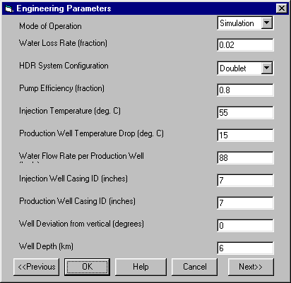
The Engineering Parameters form allows for the input of the engineering parameters of the EGS geothermal system. Also, within this menu is the option to choose the mode of operation either simulation or optimization. There are three well configuration allowed by this model, doublet, triplet, and star pattern. These have built-in assumptions concerning the ratio of injection to production wells and the geometric configuration of the wells. Among the engineering parameters that can be specified are water loss rate, pump efficiency, injection temperature, production well temperature drop, water flow rate, injection well ID, production well ID, well deviation, and well depth.
Mode of Operation refers to the type of calculations performed by the model, either Simulation, a direct calculation of the input parameters, or Optimization of certain given parameters according to an objective function of minimum breakeven electricity price.
Water Loss Rate is a ratio (in decimal units) of water loss per reservoir to production well flow used in one pass through the reservoir.
The System Configuration option configures the injection well and production well ratio and relative locations. The options are doublet, triplet, and star.
A Doublet is a system with one injection well and one production well
A Triplet is a system with one injection well and two production wells in the following pattern:
P I P
P-Production Well
I-Injection Well
A Star pattern is a system with one injection well and four producing wells in the following pattern:
    P

P  I   P

   P
P-Production Well
I-Injection Well
(Note that the well deviation from vertical must be to zero for a star configuration)
The Pump Efficiency refers to the overall efficiency (in decimal units) of the circulation pump that takes into account both thermodynamic and mechanic inefficiencies.
The Injection Temperature is the temperature (in degrees Celsius) of the fluid at the top of the injection well. This variable can be optimized.
The Production Well Temperature Drop is the temperature loss (in degrees Celsius) from conduction as the water travels to the surface.
The Water Flow Rate per Production Well refers to the mass flow rate (in kg/s) of the geofluid through a production well. This variable can be optimized.
The Injection Well Casing ID is the inner diameter (in inches) of the casing of the injection well.
The Production Well Casing ID is the inner diameter (in inches) of the casing of the production well.
The Well Deviation from Vertical is the well’s deviation from vertical (in degrees) as the well enters the reservoir. The well deviation must be zero for a star configuration. This variable can be specified or optimized when the system is a doublet or a triplet.
The Well Depth is the vertical depth (in km) of the well from the surface. This variable can be optimized.
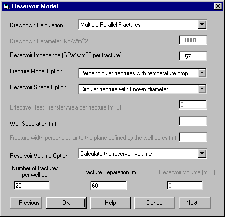
This input menu characterizes the conditions of the artificial reservoir. Three alternative thermal drawdown calculation models can be used to simulate the reservoir performance:
Multiple parallel fractures
Volumetric block
Drawdown parameter
There are also options for modeling the fracture temperature profile, modeling the shape of the reservoir and calculating the number of fractures, fracture separation, and reservoir volume.
The Drawdown Calculation is the method of calculating the decrease in heat energy output over time from the reservoir.
The Multiple Parallel Fractures model assumes one-dimensional rock conduction coupled to one-dimensional convection flow in an infinite series of parallel, equidistant, planar fractures of uniform aperture. This model was proposed by Gringarten et al. (1975).
The Volumetric Block model assumes one-dimensional linear flow in a fractured geothermal reservoir. This model was proposed by Kuo et al. (1977), Hunsbedt et al. (1978, 1983) and Irequi et al. (1978).
The Drawdown Parameter option assumes that the drawdown rate is governed by the drawdown parameter, which is the mass flow per unit of are of an individual fracture. Under this option, a value has to be specified for the drawdown parameter (in kg/sqm*s). This option was proposed by Armstead and Tester (1987).
The Reservoir Impedance is the resistance of the rock to fluid flow through a fracture (in GPa*s/cu.m per fracture)
The Fracture Model Option is the method of simulating the vertical temperature differential over the section of the reservoir in the injection well. The options are perpendicular fractures using top temperature and perpendicular fractures with temperature drop.
The option of Perpendicular fractures using top temperature assumes that the fractures are all perpendicular to the injection and producing wells and the temperature at the top of the reservoir is the value used for the whole vertical distance of the reservoir.
The option of Perpendicular fractures with temperature drop assumes that the fractures are all perpendicular to the injection and production wells and the temperature is varied according to the appropriate temperature gradient over the vertical distance of the reservoir
The Reservoir Shape Option is the method of calculating the cross-section of the fractures. The thickness of an individual fracture is assumed to be negligible in comparison with the spacing between the fractures. The options are circular fracture with known area, circular fracture with known diameter, square fracture, and rectangular fracture.
The Circular fracture with known area option uses a known heat transfer area for each fracture. With this reservoir shape option, the effective heat transfer area per fracture needs to be specified.
The Circular fracture with known diameter option uses a known diameter for an individual fracture, where fracture diameter is the distance between an injection and an production well, i.e. the well separation With this reservoir shape option, the well separation needs to be specified.
The Square Fracture option uses a known length for an individual fracture, where fracture length is the distance between an injection and a production well. With this reservoir shape option, the well separation needs to be specified.
The Rectangular Fracture option uses a known length and width for an individual fracture, where fracture length is the distance between an injection and a production well, and fracture width is the distance perpendicular to the plane defined by the well bores. With this reservoir shape option, the well separation and fracture width perpendicular to the plane defined by the well bores needs to be specified.
Effective Heat Transfer Area per Fracture (in sq.m) is the input parameter needed for the circular fracture with known area option. This variable can be optimized only when the circular fracture with known area option has been selected.
The Well Separation is the distance (in m) between an injection well and an production well. This value is needed for the circular fracture with known diameter option, the square fracture option and the rectangular fracture option. This variable can be optimized only when one of the above mentioned options has been selected.
The Fracture Width Perpendicular to the Plane Defined by the Well Bores is the dimension (in m) of an individual fracture in the direction perpendicular to the plane defined by the well bores. This needs to be specified if the rectangular fracture option is specified.
The Reservoir Volume Option allows the user to choose two of three variables to calculate the third. The three variables are number of fractures per well-pair, fracture separation, and reservoir volume.
The Number of Fractures per Well-Pair is the number of stimulated fractures between an injection and a production well. This variable can be optimized only when it is used for the calculation of either the reservoir volume or the fracture separation.
The Fracture Separation is the separation (in m) between the fractures in the stacked fractures of a well-pair. The thickness of an individual fracture is assumed to be negligible in comparison with the spacing between the fractures. This variable can be optimized only when it is used for the calculation of either the reservoir volume or the number of fractures.
Reservoir Volume is the total volume (in cu. m) within the fractures between the well-pair. This variable can be optimized only when it is used for the calculation of either the number of fractures or the fracture separation.
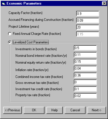
This menu specifies the general economic parameters of the project. There are two methods of evaluating the impact of time on the capital investments of the project. The first is using a simple fixed annual charge rate. The second is using the levelized life-cycle cost model, which evaluates a much richer and complex economic system. The other economic parameters that can be specified are the capacity factor, inflation rate during construction, and project lifetime.
The Capacity Factor is the ratio of the electrical energy produced by a generating unit for the period of time considered to the electrical energy that could have been produced at continuous full-power operation during the same period.
The Accrued Financing during Construction is the financial cost accrued during construction as a percentage of the total capital costs.
The Project Lifetime is the number of years of operations that the plant is amortized over .
The Fixed Annual Charge Rate is the fraction of the total capital costs annualized each year.
The Fixed AnnualCharge Rate Model calculates the break-even electricity price from the formula:
Electricity breakeven price = (annualized capital costs + annual O & M costs)/(net power produced*capacity factor)
The Levelized Cost Parameters are the parameters used by the Levelized Life-Cycle Cost Model.
The Levelized Life-Cycle Cost Model levelizes the expenditures of a project over its lifetime. The parameters used in this model are investments in bonds, nominal bond interest rate, nominal equity return rate, inflation rate, combined income tax rate, gross revenue tax rate, investment tax credit rate, and property tax rate. The algorithm used was developed in Los Alamos National Laboratory by Hardie and is documented in report LA-8909 (1981).
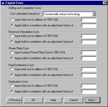
This input menu defines more specifically parameters relating to the capital costs. The total capital cost is composed of five cost categories; drilling and completion cost, reservoir stimulation cost, power plant cost, fluid distribution cost, and exploration cost. Each individual capital cost component can be input directly without using any internal correlations, or the internal correlations can be used with a factor that is multiplied to the internal value to give the final value. A value of 1 for the adjustment factor would leave the internal correlation value the same. There are three alternative technology options for calculating the drilling and completion cost; problem burdened technology, commercially mature technology, and optimized technology.
The Technology Option refers to the level of technological evolution assumed in calculating drilling and completion costs in the model. The choices for this option are problem burdened technology, commercially mature technology, and optimized technology.
Apply built-in correlation with an adjustment factor of allows for capital cost components to be calculated with the internal cost correlations and with a multiplied factor. Using a factor value of 1 calculates the capital costs solely by internal correlations.
Drilling and Completion Costs are the costs of drilling and completing the injection and production wells. There are three built-in cost levels the user may choose; problem burdened technology, commercially mature technology, and optimized technology.
Problem Burdened Technology assumes a technology level that is inductive of past experience without benefit of a learning curve.
Commercially Mature Technology uses a level of costs that will be present once a commercial infrastructure exists for these projects.
Optimized Technology uses a level of costs that assumes new technological achievements.
Reservoir Stimulation Costs are the costs of creating artificial reservoirs between the injection and production wells.
Power Plant Costs are the costs of building the power plant.
Fluid Distribution Costs are the costs of the system to distribute the fluid from the wells to the plant
Exploration Costs are the costs of initially characterizing the geothermal reservoir including the cost of hydrologic, geologic and geophysical surveys, as well as the cost of "dry holes".
Operation and Maintenance Costs
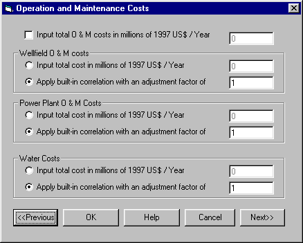
This input menu defines more specifically parameters relating to the operation and maintenance (O & M) costs. There are two ways of calculating O&M costs. One is to input a value for total O & M costs. The other way is to split the cost into wellfield, power plant, and water O&M costs. With each of these types of O&M costs, there are two ways of affecting the value. They can be input in directly without any internal correlations, or internal correlations can be used with a factor that is multiplied to the internal value to give a final value. A value of 1 for the adjustment would leave the internal correlation value the same.
Input Total O & M costs in millions of 1997 US$ / year allows the option to input the total O & M costs instead of using internal correlations.
Apply built-in correlation with an adjustment factor of allows for O & M cost components to be calculated with the internal cost correlations and with a multiplied factor. Using a factor value of 1 calculates the O & M costs solely by internal correlations.
Wellfield O & M costs is the cost of maintaining the wellfield.
Power Plant O & M Costs is the cost of operating and maintaining the power plant.
Water Cost is the cost of make-up water added in the reservoir.
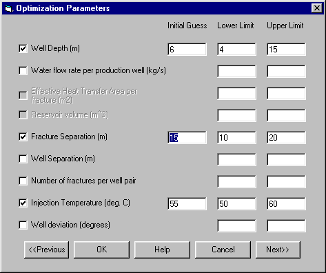
This input screen allows for initial guesses and bounds to be specified while running in optimization mode. The variables that can be optimized are:
When a box is checked for a variable to be optimized, the value for the variable originally elsewhere in the input sequence is entered into the initial guess box. This value is used to give the program an initial guess to start the optimization algorithm. According to user’s selections in the previous forms, some variables are calculated by the program. Those variables are grayed out in the optimization form. Lower limit and upper limit have to be input for each of the optimized variables. These give the optimization algorithm a bounds to work in. Any or all of these variables can be optimized for. (Note on optimizing for well depth, the upper limit is determined by the value calculated by the maximum reservoir temperature and the set of gradients).
Initial Guess is the value that the program uses to initialize the optimization.
Lower Limit is the lower bound of the range that the optimization routine can use.
Upper Limit is the upper bound of the range that the optimization routine can use.