HST.563

LAB 1: Lifecycle of a biomedical image

February 2008

http://web.mit.edu/hst.563/www/lab1/lab1 _hst563.htm

Introduction

This Lab examines the “lifecycle of an image”, from the acquisition of data using a MR imaging system, through the reconstruction of raw data into an image, and analysis of the images and inclusion into a database. The purpose is to understand how acquisition and reconstruction controls the resulting image and overall outcome of the analysis, as well as explore MR cardiac imaging techniques. An introduction to cardiac MR physics is provided as a reference. The power of biomedical imaging lies in access and control over each step in this image lifecycle.

LVfunction

The heart beats about once per second. The beat corresponds to anatomical changes in the shape of the heart chambers. The most important heart chamber for survival is the left ventricle (LV). This chamber has the most muscle, and moves the most. Its motion every heart-beat is called LV function, and is characterized by measuring the end-diastolic and end-systolic volumetric size. It can be imaged using real-time or ecg-gated MRI to measure its size.

ImagingPlanes

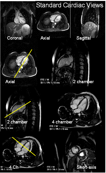
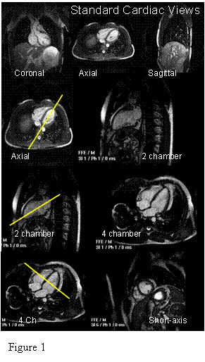
MRI, unlike CT, Nuclear imaging, PET and ultrasound, can acquire an image in any 3D slice-plane orientation. Two orthogonal slice planes will be used for analysis in this lab: the 4 chamber view and the short-axis view. Figure 1shows these two views, and their relation to the patient geometry.

Q1: What is the reason for the names of these anatomic views?

ECG-gating

For cardiac MRI, the ecg-signal obtained from chest leads can be used to time the acquisition of data. If data from a single phase of the cardiac cycle is combined, the motion is “frozen” and represents the heart’s appearance at that phase.

Breath-holding: Respiration causes motion artifacts when imaging the heart, and commonly the subject holds her breath to reduce this motion.

Q2: Should respiration be suspended at end-inspiration or end-expiration? Reasons?

Breath-held ecg-gated cine imaging shows the motion of the heart through out the heart-beat. Breath-held real-time imaging shows the motion of the heart through time.

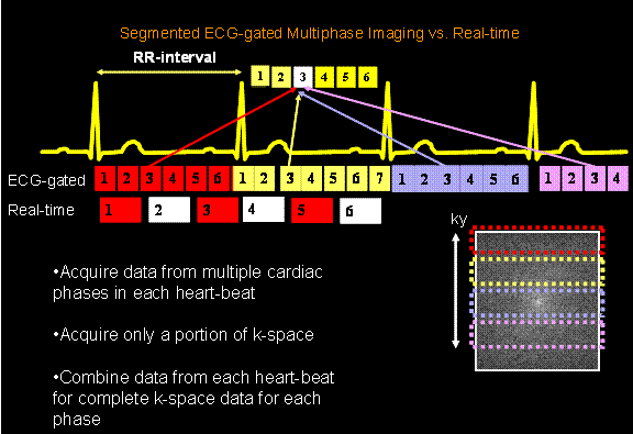
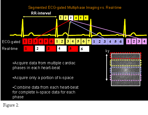
The differences between ecg-gated and real-time imaging are shown in Figure 2.

Acquisitions

We will acquire and use data from an ecg-gated segmented acquisition and a real-time acquisition. Figure 2 compares the differences in data collection for these two methods. The ecg-gated acquisition relies on periodic motion of the heart. A real-time acquisition is valuable if the heart-beat and motions are unstable. An ecg-gated acquisition acquires data over multiple heart-beats, and combines the data from all the heart-beats to form a single image. Real-time imaging is fluoroscopic, like x-ray, or ultrasound, acquiring a complete image repeatedly over time. Both types of images provide quantitative information on changes in LV size and shape during the cardiac cycle. Again, these changes are called “LV function”.

Lab Overview

The organization for this lab is as follows:

Part I: Image Acquisition

We will demonstrate breath-held and ecg-gated cardiac MRI during the lab and will providea dataset for the lab writeup.

Part II: Image Reconstruction

We will reconstruct the MR images from raw coil signal data using Fourier transforms and decimation, coil combination and some image processing methods.

Part III: Image Analysis

We will perform volumetric analysis of the heart images.

Part IV: Creating Dicoms

Dicom is the standard format used for medical images and stands for Digital Imaging and Communications in Medicine. We will convert our Matlab images into the DICOM format.

Guidelines for Laboratory Report

Your laboratory report should contain answers to the questions specified in red. Do not repeat the lab instructions and avoid lengthy introductions. Your report should not exceed 6 pages. Include the images that you have reconstructed, and how the analysis was performed. Conclude your report with a few sentences summarizing what you learned in the lab.

Part I: Image acquisition

The volunteer will be placed in the scanner. Four sets of data will be acquired, in addition to localizers: cine and ecg-gated imaging in the 4 chamber and short-axis views. Real-time data will also be acquired with a temporal resolution of 180 ms, and a FOV of 320 mm, in the 4 chamber and short-axis views.

Q3: Describe how the subject is prepared for scanning.

During the acquisition of data, we will save the raw data, find it saved to disk on the scanner, and also export some dicom images for use in the lab.

PartII: Image Reconstruction

Data for this part are found in the directory: athena.mit.edu/course/other/hst.563/lab1. For remote users, use SFTP via athena.dialup.mit.edu to access this folder.

The cine ecg-gated raw data sets have 5 coils, and 16 cardiac phases, and the k-space data matrix size is 320 x160 (Nx x Ny). The real-time raw data sets have 5 coils, and16 cardiac phases, and the k-space data matrix size is 256 x 64.

The naming convention is this: 101_coil3_phase4.sig contains the k-space data for data set 1 (ecg-gated cine), coil 3 and cardiac phase 4.

Extract data (using extract_kspace_hst.m): Each k-space must be reconstructed with an FFT. Read the k-space data into a matrix—Matlab code is provided for this. For reading k-space data from a raw datafile, the vendor must provide the format. The k-space data is usually stored with a Header, followed by raw data from phase-encoding 1-N. Since k-space is complex, each phase-encoding requires storage for two floating point numbers (real and imaginary signals). Guess at the number of bytes for storing the floating point numbers.

Q4: Find the size of the raw data, for an ecg-gated data set, 1st coil, 1st phase. What is the header size? (Hint, look at lecture 4).

Q5: Calculate the size of each floating point in bytes—does it work out?

Recon Overview

1. Read in raw data

2. Decimate kspace data (MR data usually comes over sampled by a factor of 2 in the frequency encoding dimension, e.g. 320 x 160 here, although the requested data is 160 x 160)

3. Zero fill kspace data—to the nearest factor of 2—interpolation makes the images look better.

4. For the real-time images, perform the view-sharing of k-space.

5. FFT the data.

6. Fix the aspect ratio i.e. for the real-time data the FOV in the y-direction is ½ of the FOV in the x-direction, so it would be helpful to keep this aspect ratio in the images.

7. Combine images from multiple coils.

8. Perform this for each phase of the cardiac cycle.

FFT data

FTSHIFT: this function shifts a matrix by half in both directions, and is useful for centering k-space or image space, but is a little DANGEROUS, because it sometimes causes unexpected effects...

Q6: Write down the 1D Fourier shift theorem (for shifting ½ FOV away), and explain what happens to data when: ifft(fft(fftshift(data))

Hint: When reconstructing raw data always view the raw data during intermediate stages—and it’s helpful to view real and imaginary data separately.

Decimation

The data set includes a 320 Nx k-space points. This data corresponds to a 640 mm FOV (double FOV), the kspace must be “decimated” by a factor of 2 in the Nx direction.

Q7: If you decimate by taking every other point in kx-space, will this work? What will happen?

Decimate and fft data for each coil and phase (use fft, ifft, fft2, ifft2, fftshift)

Combine data from each coil

For each cardiac phase, the coil image data is combined together using a weighted sum, with j the coil index.

(1)

Combine coil images for each phase (Equation 1), where the weightings at each pixel for each coil are estimated as the signal from the coil itself.

Sliding window recon for real-time data

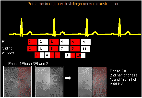
For the real-time data set, reconstruct with FFT, and also using a sliding window reconstruction (see Foo et al, Figure 3), or mathematically, to construct an intermediate kspaced data set (Sint(kx,ky), use data acquired for phase n, and phase n+1.

(2)

where

This addition of two parts of k-space from successive phases to create an “intermediate phase” is called sliding window reconstruction, or “view sharing” because each k-space line is called a view. Note: This sliding window method assumes that ky-space was collected in time in a sequential order, e.g, for 8 views:

Phase1 -4, -3, -2, -1, 0, 1, 2, 3, Phase2 -4, -3, -2, -1, 0, 1, 2, 3,

Then the intermediate phase is constructed from:

(Phase 1) 0, 1, 2, 3, (phase 2), -4, -3, -2, -1

Q8: Mathematically is there another way to do this, which would result in a similar temporal interpolation?

Reconstruct all phases for each data set. Then use sliding window reconstruction to reconstruct the real-time data sets with 2x the number of phases. (Equation 2).

Part III:Image Analysis

After reconstruction, you will have three sets of images, each in the 4ch and 2ch orientations; each is a series of images showing heart movement throughout the cardiac cycle.

Set 1: Cine ecg-gated 4ch and 2ch (16 phases, 37 ms temporal resolution).

Set 2: Real-time 4chand 2ch (16 phases, 180 ms temporal resolution).

Set 3: Sliding window-reconned real-time 4ch and 2ch (31 phases).

Q9: What is the temporal resolution of Set 3?

Identify frames of end-diastole and end-systole. Systole is defined as the image with the smallest LV cavity. End-diastole is defined as immediately after the QRS interval. For the real-time imaging data set, choose a reasonable frame.

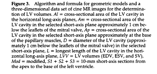
Manually planimeter the areas of LV blood in the 4 chamber and short-axis views for end-systole, end-diastole, with each data set. Please show an example of this planimetry in your report. These are areas, and must be converted from pixel to true areas by multiplication by pixel size (don’t use slice thickness).

Use biplane ellipsoid method (Figure 3, from Foo et al) and the roipoly.m for calculating LV volumes at end-systole and end-diastole.

Q10: What is the conversion factor – pixels to mm2?

Q11: Will you include or exclude the papillary muscles in your measurements—provide pros and cons for each?

Q12: Fill in the Tables:

	4 chamber area		Shax area
	End-Diastole	End-Systole	End-Diastole	End-Systole
Data set 1
Data set 2
Data Set 2 sliding window

	End diastolic vol	End systolic vol	Ejection fraction
Data set 1
Data set 2
Data set 2 – Sliding window

Q13: Calculate EF = (EDV-ESV)/EDV

Q14: How does this EF compare to normal values? How do EFs differ for each data set?

Part IV: Creating Dicoms

Creating Dicom images from the images that have been reconstructed “offline” is important, because the images can then be used by any commercial image viewer, and subjected to advanced image processing. Dicoms are very easily created using a template, by stripping the dicom “header” off of an already existing commercially created image.

The general steps are:

Use a template image, strip off the header
Modify the header with new values as needed
Write the image data and the new header to a new image file
Import the new image

Please use the DICOMs provided as the template for the DICOM header.

Q15: Using one of the dicom files, write a tiny matlab script to read the signature of the DICOM (see Lecture notes and Reference) “D” “I” “C” “M”. Include this script in your lab report.

Create dicoms for images reconstructed with sliding window recon. In Matlab:

header_info = dicominfo(name0); dicomwrite(image2, name1,header_info);

Q16: Create new DICOMS for the sliding window reconstructed images, which must be submitted with your report (electronic copies, burn to CD or email TAs).

Questions

Below is a list of the questions asked throughout the lab: