Tabulating values of the Riemann-Siegel Z function along the critical line

Abstract

This project makes three main contributions:

Tabulation of 2,354,000,000 values of the Riemann-Siegel Z function in the domain 2.7 < t < 29,143,636.6, and tabulation of 5,000,000 values of the Riemann-Siegel Z function in neighborhood of the trillionth (10¹²th) zero.
Tabulation of 47 terms of the remainder series of the Riemann-Siegel formula.
Tabulation of the coefficients of Chebyshev polynomials for the first 6 terms of the remainder series of the Riemann-Siegel formula.

Introduction

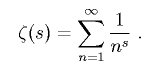
Riemann's zeta function is defined as the analytic continuation of

$\zeta(s)=\sum_{n=1}^{\infty}\frac{1}{s^n}$

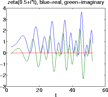
to the entire complex plane. (The series itself only converges for Re(s) > 1.) The Riemann conjecture states that all non-trivial zeros of the zeta function occur along the line Re(s) = 0.5. This line is known as the critical line.

The values (the real and imaginary parts) of the zeta function evaluated along the critical line oscillate around zero, as the plot below illustrates.

I was inspired from the visual appearance of these plots to try to produce a sound file of the zeta function along the critical line. A similar attempt was made by Robert Munafo .

Therefore, the real motivation for this project is artistic . I just wanted to hear what it sounded like (and to take advantage of a computational resource that I would not likely have again any time in the near future) . I was not out to discover any deep mathematical revelations, although the tabulations may be useful to other mathematicians for that endeavor. I am not attempting to solve any particularly difficult or interesting parallel computer programming problem; the parallelization implemented was of the "embarrassingly" variety and relatively trivial.

To borrow a quote from George Mallory, I performed this calculation of the Z function "because it's there."

Useful links

Riemann-Siegel formula

The Riemann-Siegel formula is an approximation formula for the Zeta function specifically on the critical line. Evaluation of the formula requires O(t^1/2) operations to evaluate a single value of Zeta(0.5 + t *i) . This is in contrast to the faster Odlyzko - Schönhage method, which requires amortized O(t^ε) operations per evaluation (where ε can be made arbitrarily small at the cost of a higher space requirement) . However, the Odlyzko - Schönhage is very complicated, so I chose not to implement it.

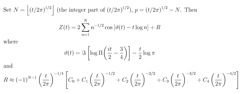
The Riemann-Siegel formula (excerpted from (Pugh 1998)) for calculating Zeta(0.5 + t * i) for t > 0 is:

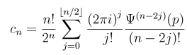
Note that the calligraphic I (

) function signifies "take the imaginary part" . The capital Pi (Π) function is Π(s) = Gamma(s+1) . The superscripts above the Psi (Ψ) functions signify repeated differentiation with respect to p .

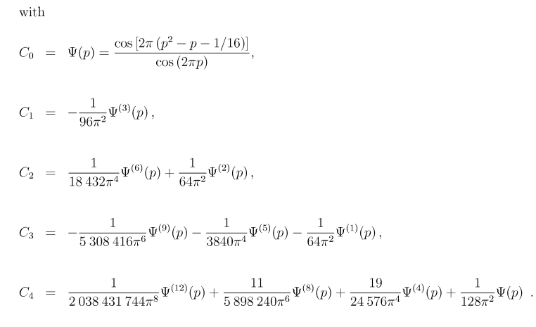
The C_n functions are undefined at p = 0.25 and p = 0.75. The values at those points are the limiting values (from either side) .

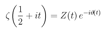
And finally, Zeta(0.5 + t * i) is calculated as:

Note that the sum in the Z(t) function is the only computationally expensive part of the calculation. After Z(t) is known, Zeta(0.5 + t * i) can be calculated easily. Therefore, the remainder of this project deals with tabulating values of the Z function, and not the Zeta function. (The tabulated values of Z require half as much space to store because they are not complex.) Also, the zeros of the Z function coincide with the zeros of the Zeta function along the critical line.

Verifying the remainder terms

The first part of this project was to verify (and extend) the remainder terms (i.e., the C_n functions) of the Riemann-Siegel formula. Both references to the formula I found on the web, namely (Pugh 1998) and Mathworld , both referenced Edwards's 1974 book for the remainder terms. It was conceivable that an arithmetic or typographical error could have been propagated through the documents.

Note that I am verifying the low-level arithmetic and algebra of the derivation of the remainder terms, and not the high-level complex analysis upon which the Riemann-Siegel formula is based.

My verification followed the derivation described in (Pugh 1998) sections 3.8-3.9. Note that there is one typographical error and one confusing point in his derivation, see my e-mail conversation with him. The formulae below have the typographical error corrected.

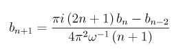
The first step is to calculate the sequence b_n from the following recurrence:

where b_-2 = 0, b_-1 = 0, and b₀ = 1.

The second step is to calculate the sequence c _n from the following formula:

My Haskell program zetaR.el.hs calculates these symbolic expressions and produces output which can be fed into Matlab. (The programming language Haskell, with its built in support for arbitrary precision arithmetic on rationals and "lazy" infinite lists (used to implement infinite series) was quite useful for this part of the project.) I calculated the first 201 terms (up to n = 200) of each sequence.

The remainder of the calculation was done with Matlab's symbolic toolbox, and is documented in the Matlab diary file 47-coefficients.txt .

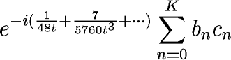
The following product is formed:

$e^{-i(\frac{1}{48t}+\frac{7}{5760t^3}+\cdots)}\sum_{n=0}^{K}b_nc_n$

into which we substitute t = 2π/ω² , and the notation "e^X" denotes the Taylor expansion of the exponential function about zero.

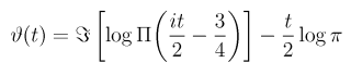
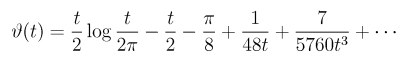
The series inside the parenthesis are the negative order terms of the series expansion of the Theta function:

The series follows from the Stirling approximation of the Gamma function. Coaxing this series out of Matlab was somewhat involved, the line in the diary which produces 150 terms of the series is gg=sym(maple('asympt',rr,x,150))

Finally, after forming the product, we can collect by powers of ω , (the Matlab command was maple('coeff',infisubs*psum,omega,i)) , yielding the n-th remainder term as the coefficient to ωⁿ . I ran this calculation until Maple broke: For the 47th term, it died with an error message complaining about "integer too large in context" .

In the diary file, the notation Pn , e.g. P7 , denotes the n-th derivative of the Psi (Ψ) function. The first few terms beyond those given in Pugh's thesis are:

C₅ = -1/978447237120/pi^10*P15 - 7/849346560/pi^8*P11 - 5/3072/pi^4*P3 - 901/82575360 /pi^6*P7
C₆ = 1/563585608581120/pi^12*P18 + 18889/237817036800/pi^8*P10 + 17/652298158080/pi^10*P14 + 367/7864320/pi^6*P6 + 5/2048/pi^4*P2
C₇ = -5/2048/pi^4*P1 - 407/2621440/pi^6*P5 - 6649/11890851840/pi^8*P9 - 2131/5707608883200/pi^10*P13 - 1/15655155793920/pi^12*P17 - 1/378729528966512640/pi^14*P21
C₈ = 1/290864278246281707520/pi^16*P24 + 11153/8766887244595200/pi^12*P16 + 26405/8455716864/pi^8*P8 + 427/1048576/pi^6*P4 + 41/32768/pi^4*P0 + 88651/22830435532800/pi^10*P12 + 23/180347394745958400/pi^14*P20

More terms are given at the end of the diary file . C₅ agrees with a formula given at Mathworld . C₆ through C₄₆ have not been published before to the best of my knowledge.

This project would have benefitted from a parallelized symbolic computation package. The timings of the symbolic calculations are included in the diary file. Some of the commands listed in the diary took longer than 10 minutes. The most time-consuming calculation (not shown in diary file) was the dot product Σb_nc_n, which took over 30 minutes.

The directory remainder_terms/ contains Matlab scripts used in the computation.

Chebyshev polynomials for the remainder terms

It would be very unwise to implement the remainder terms exactly as the expressions which result from the symbolic computations above. The high derivatives of the Psi function yield extremely long expressions, which result in numerical instability, especially near the singular points p = 0.25 and p = 0.75.

The wise thing to do is to symbolically compute some series expansion of the remainder terms. Pugh, in his master's thesis, chose a Taylor expansion (around p = 0.5) . This project does slightly better by computing a Chebyshev polynomial for each of the remainder terms.

(Although, since very little of the computation time is spent on evaluating the remainder terms, the computation time saved by using a Chebyshev polynomial instead of a Taylor polynomial is negligible.)

The algorithm described in Numerical Recipes was used to generate the Chebyshev coefficients. The calculations were carried out with 200 digits of precision using the vpa command in Matlab. These computations were extremely time consuming as well, taking on the order of 30 minutes per remainder term (the higher order terms, e.g., C₆ , took a long time to calculate) . Fortunately, the task is embarrassingly parallel and was carried out on 6 Athena computers, one for each term calculated. With these coefficients published here, hopefully no one will have to calculate them again.

The Chebyshev coefficients for the first 6 remainder terms (namely C₀ through C₅) are given in coff-all.h . There are 101 coefficients for each term. For my computation, I truncated the polynomial to 20 terms.

Plots of the first six remainder terms look as follows:

The directory cheby/ contains Matlab scripts used in this computation.

Implementation details

We now discuss a few of the implementation details of the ideas presented above.

Verifying correctness

For low values of t , the implementation was verified by comparing with Matlab's zeta function. Matlab's zeta function uses an algorithm which requires O(t) operations per point, so can only be used for low values of t.

For high values of t , I evaluated Z at the 10,000 zeros in the neighborhood of the trillionth zero previously computed by A. Odlyzko. If my program is implemented correctly, all of these evaluations should be near zero, which they were. The maximum deviation from zero was 1.4235e-05, and the root-mean-square (RMS) deviation over all 10,000 zeros was 9.7010e-07.

Scaling horizontally

The density of the zeros of the Z function (and consequently the Zeta function) increases as O(log t). This "sort of" follows from the "t/2 log (t/(2 pi))" leading term of the series expansion of the Theta function above.

Recall that the purpose of this project is to produce a sound file. The effect of the increasing density of the sound file is that the frequency of the sound will increase logarithmically. Unfortunately, this will make the sound file annoying or painful to listen, so we must counteract this effect.

The countermeasure I implemented was to scale the t axis by 1/log t . Specifically:

Let N be the sample number, where N= 0,1,2,...
Let y = 3+ (N/4)
Let t = y /log y
Then, the N-th sample is the value of Z(t) .

These parameters were chosen so that the sound file is not too annoying to listen, when played at 44.1 kHz. The frequency does slowly change over the course of the sound file. This is because x / log x is not an exact inverse of x * log x .

Scaling Vertically

The sound file stores samples as 16-bit signed integers, so we must scale the value returned by the Z function into the range -32768 ... 32767.

The maximum absolute value of the Z function encountered in the first 2,354,000,000 samples was 74.2677, which occurred at t = 15457423.7117588, or sample number 1207244046. Therefore, the scaling constant was chosen to be 256. Note that the reciprocal of the scaling constant can be exactly represented in binary, so the value of Z can be reconstructed exactly (up to the limit of roundoff error) .

The maximum absolute value of the Z function encountered in the neighborhood of the trillionth zero was -134.2658, which occurred at t = 267653412338.13435665, or sample number 31801774248668. Therefore, the scaling constant was chosen to be 128.

It is interesting to examine these peaks with Glen Pugh's Zeta plotter .

Unfortunately, these peaks were discovered by a two pass algorithm: First compute all the values and determine the min and max, then compute all the values again scaling by the right constant.

Extreme values of Z occur quite rarely, so the sound file is rather quiet as a result.

Key optimization

Almost all of the computation time (roughly 98%) is spent in an inner loop which computes the sum of the Riemann-Siegel formula. This inner loop has two key optimizations. The relevant lines of code are:

for (int n = 1; (n <= N); ++n) {

sumZ += (cosl ((theta_t - (t * lookup[n]._logl))) / lookup[n]._sqrtl)

}

The values of log and sqrt are computed via lookup table.
The lookup table is stored as an array of records (as opposed to parallel arrays) , so that entries for _logl and _sqrtl will end up on the same cache line.

These two optimizations more than doubled the speed of my program.

Parallel Execution

Multiple evaluations of the Z function is an embarrassingly parallel task. My program, written with MPI, has a parent process which deals out small chunks of 1,000,000 samples of the domain to each of the child processes. As each child process finishes, it is assigned a new chunk. The total CPU time consumed in calculating the first 2,354,000,000 samples was approximately 100 hours, which was spread out over 6 to 9 processors. (The entire computation was not done in a single run.) It is interesting to note that the computation ran approximately at "real time" because the audio file produced is 14 hours long.

A mildly clever innovation I implemented was to prevent a multi-gigabyte temporary file from forming as the calculation progressed. As each chunk is completed, it is immediately losslessly compressed into the FLAC audio format, which saves storage by a factor of 6. The compression was performed by a Perl script which periodically polled the file system (every 10 minutes) looking for completed chunks.

The CPU time consumed for tabulating 5,000,000 values in the neighborhood of the trillionth zero was about 35 hours, spread out over 6 processors. The chunk size was 10,000. Clearly high values take longer to calculate.

Tabulations

This project produced two tabulations of the Riemann-Siegel Z function (from which the values of the Riemann Zeta function along the critical line Re(s) = 0.5 can easily calculated) which may be useful to curious mathematicians, or entertaining to curious listeners. These tabulations are stored as audio files. For completeness, the issues of horizontal and vertical scaling mentioned in the previous section will be repeated here. The tabulations produced are:

A tabulation from sample number N=0 to sample number N=2,353,999,999. The domain and range of the Z values stored in the file are:
- Let N be the sample number, where N= 0,1,2,...
- Let y = 3+ (N/4)
- Let t = y /log y
- Then, the N-th sample has the value of 256* Z(t) , rounded to the nearest 16-bit integer
Therefore, the range of evaluated values is approximately 2.7 < t < 29,143,636.6.
A downloadable tabulation from sample number N=31801772196387 to N=31801772196387+4999999. The domain and range of the Z values stored in the file are:
- Let N be the sample number, where N= 31801772196387, 31801772196388, 31801772196389, ...
- Let y = 3+ (N/4)
- Let t = y /log y
- Then, the N-th sample has the value of 128* Z(t) , rounded to the nearest 16-bit integer
Therefore, the range of evaluated values is approximately 2.67653395646999e+11 < t < 2.67653436311838e+11 .

The tabulations are losslessly compressed into the FLAC audio format. The FLAC command line to uncompress the files to stdout is flac -d -c -fr -fl filename.flac , (You may wish to change the -fl flag to -fb if you have a big-endian machine. Intel machines are little-endian.) Note that the first tabulation would produce a 4.4 gigabyte uncompressed file, which might break your operating system's limit of 2 GB files. In such a case, you should pipe the output directly to whatever analysis program you are running.

Obtaining the long tabulation

If you are interested in obtaining the first long tabulation of 2.354 billion values, please contact me at my permanent e-mail address kenta at cs dot stanford dot edu . The tabulation is approximately 800MB compressed. The easiest way to transfer the file would be for you to set up an anonymous FTP account where I can dump the file.

Audio files

In the limited space of my account are contained riemann_low.mp3 which is the initial part of the first tabulation, and riemann_hi.mp3 which is the entirety of the second tabulation. It is interesting to note that these files sound radically different. Over the course of a trillion zeros, the sound of the Z function slowly changes. The sound of the Z function does capture the sound of the Zeta function: My first file of the Z function sounds quite similar to Robert Munafo's calculation of the Zeta function.

I also have available as a 350MB MP3 file the 2,354,000,000 sample tabulation. Here I reveal the that the number 2,354,000,000 was not chosen at random: The audio file, played at 44.1 kHz, plays for 14.8 hours, or 0.618 day. The ratio 0.618 is approximately the golden ratio, which is aesthetically the "most irrational" number. That is, if the sound file is played continuously repeatedly for many days, but the listener is only awake or present for certain hours of the day, the ratio 0.618 maximizes the "coverage" heard on different days.

I have not yet listened to the file in its entirety. Unfortunately, the ambient noise produced by my computer (by the fan and the hard drives) masks the sound a lot, so it is recommended that the audio file (350 MBmb) be written or downloaded to a portable MP3 device (such as a MP3 CD player) and played. Please contact me at the address given above to obtain the file.

Analyses

The following are some simple analyses of the Z tabulations. They only represent examples of things which could be done by curious mathematicians seeking to investigate the Riemann Zeta function empirically. For brevity, the tabulation from 0 to 2,354,000,000 will be referred to as the LOW dataset, and the tabulation in the region of the trillionth zero will be referred to as the HIGH dataset.

	LOW	HIGH
Samples	2354000000	5000000
Min	-68.13	-134.27
Max	74.27	109.58
Mean	-1.1331e-05	0.0017698
Root Mean Square value	3.9442	5.0539
Approx. num zeros	66548266	158297
Largest spacing between zeros	159 samples	114 samples
Mean spacing between zeros	35.373 samples	31.586 samples

The number of zeros is approximate because of the 16 bit precision of the data. The function may creep just barely above (or below) zero and not cause a sign change.

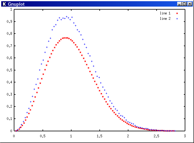
Distribution of the spacings between zeros

The following plot gives the probability density of the spacings of the zeros for the two data sets. The mean spacing has been normalized to unity for each data set (separately) . Note that the sample data was already scaled horizontally by a factor of log t (that is, the density of zeros) . The LOW data set is given in red as "line 1 *" , and the HIGH data set is given in blue as "line 2 +" .

The LOW data set has a long tail which extends off the right hand edge of the graph. The image above is quite similar to a computation performed by Odlyzko in the region of the 10¹⁶th zero (excerpted from Odlyzko 2001) .

Fourier Transform

The following two plots are the power spectrum (on a logarithmic scale) of the LOW data set of 2²⁴ samples between sample number 168442784 and sample number 185219999. The peak frequency can be clearly heard in the audio file.

The second plot is a zoom-up of the peak frequency, showing an interesting crown-like structure.

This last plot is the power spectrum of the HIGH data set.

The Fourier transforms were performed with FFTW . The size 16,777,216 transform took 17.5 seconds to compute.

This page is best viewed with a standards-compliant browser such as Mozilla (with which you may wish to turn on the Site Navigation Bar in the View Menu) . The internal anchors which are used in the Table of Contents are known not to work for older versions of Netscape, which do not support the ID attribute on the DIV tag.

References

Edwards, H. M. Riemann's Zeta Function. New York: Academic Press, 1974.
Fast algorithms for multiple evaluations of the Riemann zeta function, A. M. Odlyzko and A. Schoenhage, Trans. Am. Math. Soc., 309 (1988) , pp. 797-809.
The 10^22-nd zero of the Riemann zeta function, A. M. Odlyzko. Dynamical, Spectral, and Arithmetic Zeta Functions, M. van Frankenhuysen and M. L. Lapidus, eds., Amer. Math. Soc., Contemporary Math. series, no. 290, 2001, pp. 139-144.
"The Riemann-Siegel formula and large scale computations of the Riemann Zeta function" , Glendon Pugh, Master's thesis, University of British Columbia, 1998