Python is an interpreted, interactive, object-oriented programming language. It is often compared to Tcl, Perl, Scheme or Java.
Python combines remarkable power with very clear syntax. It has modules, classes, exceptions, very high level dynamic data types, and dynamic typing. There are interfaces to many system calls and libraries, as well as to various windowing systems (X11, Motif, Tk, Mac, MFC, wxWidgets). New built-in modules are easily written in C or C++. Python is also usable as an extension language for applications that need a programmable interface.
The Python implementation is portable: it runs on many brands of UNIX, on Windows, OS/2, Mac, Amiga, and many other platforms.
Some of Python's notable features:
We will not discuss the specifics of Python here but instead refer the reader to the Python website. Also see Dive Into Python - Python from novice to pro
lpsolve is callable from Python via an extension or module. As such, it looks like lpsolve is fully integrated with Python. Matrices can directly be transferred between Python and lpsolve in both directions. The complete interface is written in C so it has maximum performance. The whole lpsolve API is implemented with some extra's specific for Python (especially for matrix support). So you have full control to the complete lpsolve functionality via the lpsolve Python driver. If you find that this involves too much work to solve an lp model then you can also work via higher-level script files that can make things a lot easier. See further in this article.
Python is ideally suited to handle linear programming problems. These are problems in which you have a quantity, depending linearly on several variables, that you want to maximize or minimize subject to several constraints that are expressed as linear inequalities in the same variables.ĀIf the number of variables and the number of constraints are small, then there are numerous mathematical techniques for solving a linear programming problem. Indeed these techniques are often taught in high school or university level courses in finite mathematics.ĀBut sometimes these numbers are high, or even if low, the constants in the linear inequalities or the object expression for the quantity to be optimised may be numerically complicated in which case a software package like Python is required to effect a solution.
To make this possible, a driver program is needed: lpsolve55.pyd/lpsolve55.so. This driver must be put in a directory known to Python and Python can call the lpsolve solver.
This driver calls lpsolve via the lpsolve shared library (lpsolve55.dll under Windows and liblpsolve55.so under Unix/Linux) (archive lp_solve_5.5.2.5_dev.zip/lp_solve_5.5.2.5_dev.tar.gz). This has the advantage that the lpsolve driver doesn't have to be recompiled when an update of lpsolve is provided. The shared library must be somewhere in the Windows path.
So note the difference between the Python lpsolve driver that is called lpsolve and the lpsolve library that implements the API that is called lpsolve55.
There are also some Python script files (.py) as a quick start.
See Install the lpsolve driver for the installation of these files.
To test if everything is installed correctly, enter the following in the Python command window.
>>> from lpsolve55 import *
>>> lpsolve()
If it gives the following, then everything is ok:
lpsolve Python Interface version 5.5.0.6
using lpsolve version 5.5.2.5

Usage: [ret1, ret2, ...] = lpsolve('functionname', arg1, arg2, ...)
If you get the following:
This application has failed to start because lpsolve55.dll was not found.
Re-installing the application may fix this problem.
Or (Unix/Linux):
liblpsolve55.so: cannot open shared object file: No such file or directory.
Then Python can find the lpsolve driver program, but the driver program cannot find the lpsolve library
that contains the lpsolve implementation.
This library is called lpsolve55.dll under Windows and liblpsolve55.so under Unix/Linux.
Under Windows, the lpsolve55.dll file must be in a directory that in the PATH environment variable.
This path can be shown via the following command in Python: !PATH
It is common to place this in the WINDOWS\system32 folder.
Under Unix/Linux, the liblpsolve55.so shared library must be either in the directories /lib or /usr/lib or in
a directory specified by the LD_LIBRARY_PATH environment variable.
In the following text, >>> before the Python commands is the Python prompt. Only the text after >>> must be entered.
To call an lpsolve function, the following syntax must be used:
>>> [ret1, ret2, ...] = lpsolve('functionname', arg1, arg2, ...)
The return values are optional and depend on the function called. functionname must always be enclosed between single quotes to make it alphanumerical and it is case sensitive. The number and type of arguments depend on the function called. Some functions even have a variable number of arguments and a different behaviour occurs depending on the type of the argument. functionname can be (almost) any of the lpsolve API routines (see lp_solve API reference) plus some extra Python specific functions. Most of the lpsolve API routines use or return an lprec structure. To make things more robust in Python, this structure is replaced by a handle or the model name. The lprec structures are maintained internally by the lpsolve driver. The handle is an incrementing number starting from 0. Starting from driver version 5.5.0.2, it is also possible to use the model name instead of the handle. This can of course only be done if a name is given to the model. This is done via lpsolve routine set_lp_name or by specifying the model name in routine read_lp. See Using model name instead of handle.
Almost all callable functions can be found in the lp_solve API reference. Some are exactly as described in the reference guide, others have a slightly different syntax to make maximum use of the Python functionality. For example make_lp is used identical as described. But get_variables is slightly different. In the API reference, this function has two arguments. The first the lp handle and the second the resulting variables and this array must already be dimensioned. When lpsolve is used from Python, nothing must be dimensioned in advance. The lpsolve driver takes care of dimensioning all return variables and they are always returned as return value of the call to lpsolve. Never as argument to the routine. This can be a single value as for get_objective or a matrix or vector as in get_variables. In this case, get_variables returns a 4x1 matrix (vector) with the result of the 4 variables of the lp model.
Note that you can get a usage of lpsolve, its arguments and the constants that it defines by entering the following in Python:
>>> import lpsolve55
>>> help(lpsolve55)
Help on module lpsolve55:

NAME
    lpsolve55

FILE
    c:\python24\lib\site-packages\lpsolve55.pyd

CLASSES
    exceptions.Exception
        lpsolve.error

    class error(exceptions.Exception)
     |  Methods inherited from exceptions.Exception:
     |
     |  __getitem__(...)
     |
     |  __init__(...)
     |
     |  __str__(...)

FUNCTIONS
    lpsolve(...)
        lpsolve('functionname', arg1, arg2, ...) ->  execute lpsolve functionname with args

DATA
    ANTIDEGEN_BOUNDFLIP = 512
    ANTIDEGEN_COLUMNCHECK = 2
    ANTIDEGEN_DURINGBB = 128
    ANTIDEGEN_DYNAMIC = 64
    ANTIDEGEN_FIXEDVARS = 1
    ANTIDEGEN_INFEASIBLE = 32
    ANTIDEGEN_LOSTFEAS = 16
    ANTIDEGEN_NONE = 0
    ANTIDEGEN_NUMFAILURE = 8
    ANTIDEGEN_RHSPERTURB = 256
    ANTIDEGEN_STALLING = 4
    BRANCH_AUTOMATIC = 2
    BRANCH_DEFAULT = 3
    BRANCH_CEILING = 0
    BRANCH_FLOOR = 1
    CRASH_LEASTDEGENERATE = 3
    CRASH_MOSTFEASIBLE = 2
    CRASH_NONE = 0
    CRITICAL = 1
    DEGENERATE = 4
    DETAILED = 5
    EQ = 3
    FEASFOUND = 12
    FR = 0
    FULL = 6
    GE = 2
    IMPORTANT = 3
    IMPROVE_BBSIMPLEX = 8
    IMPROVE_DUALFEAS = 2
    IMPROVE_NONE = 0
    IMPROVE_SOLUTION = 1
    IMPROVE_THETAGAP = 4
    INFEASIBLE = 2
    Infinite = 1e+030
    LE = 1
    MSG_LPFEASIBLE = 8
    MSG_LPOPTIMAL = 16
    MSG_MILPBETTER = 512
    MSG_MILPEQUAL = 256
    MSG_MILPFEASIBLE = 128
    MSG_PRESOLVE = 1
    NEUTRAL = 0
    NODE_AUTOORDER = 8192
    NODE_BRANCHREVERSEMODE = 16
    NODE_BREADTHFIRSTMODE = 4096
    NODE_DEPTHFIRSTMODE = 128
    NODE_DYNAMICMODE = 1024
    NODE_FIRSTSELECT = 0
    NODE_FRACTIONSELECT = 3
    NODE_GAPSELECT = 1
    NODE_GREEDYMODE = 32
    NODE_GUBMODE = 512
    NODE_PSEUDOCOSTMODE = 64
    NODE_PSEUDOCOSTSELECT = 4
    NODE_PSEUDONONINTSELECT = 5
    NODE_PSEUDORATIOSELECT = 6
    NODE_RANDOMIZEMODE = 256
    NODE_RANGESELECT = 2
    NODE_RCOSTFIXING = 16384
    NODE_RESTARTMODE = 2048
    NODE_STRONGINIT = 32768
    NODE_USERSELECT = 7
    NODE_WEIGHTREVERSEMODE = 8
    NOFEASFOUND = 13
    NOMEMORY = -2
    NORMAL = 4
    NUMFAILURE = 5
    OPTIMAL = 0
    PRESOLVED = 9
    PRESOLVE_BOUNDS = 262144
    PRESOLVE_COLDOMINATE = 16384
    PRESOLVE_COLFIXDUAL = 131072
    PRESOLVE_COLS = 2
    PRESOLVE_DUALS = 524288
    PRESOLVE_ELIMEQ2 = 256
    PRESOLVE_IMPLIEDFREE = 512
    PRESOLVE_IMPLIEDSLK = 65536
    PRESOLVE_KNAPSACK = 128
    PRESOLVE_LINDEP = 4
    PRESOLVE_MERGEROWS = 32768
    PRESOLVE_NONE = 0
    PRESOLVE_PROBEFIX = 2048
    PRESOLVE_PROBEREDUCE = 4096
    PRESOLVE_REDUCEGCD = 1024
    PRESOLVE_REDUCEMIP = 64
    PRESOLVE_ROWDOMINATE = 8192
    PRESOLVE_ROWS = 1
    PRESOLVE_SENSDUALS = 1048576
    PRESOLVE_SOS = 32
    PRICER_DANTZIG = 1
    PRICER_DEVEX = 2
    PRICER_FIRSTINDEX = 0
    PRICER_STEEPESTEDGE = 3
    PRICE_ADAPTIVE = 32
    PRICE_AUTOPARTIAL = 256
    PRICE_HARRISTWOPASS = 4096
    PRICE_LOOPALTERNATE = 2048
    PRICE_LOOPLEFT = 1024
    PRICE_MULTIPLE = 8
    PRICE_PARTIAL = 16
    PRICE_PRIMALFALLBACK = 4
    PRICE_RANDOMIZE = 128
    PRICE_TRUENORMINIT = 16384
    PROCBREAK = 11
    PROCFAIL = 10
    SCALE_COLSONLY = 1024
    SCALE_CURTISREID = 7
    SCALE_DYNUPDATE = 256
    SCALE_EQUILIBRATE = 64
    SCALE_EXTREME = 1
    SCALE_GEOMETRIC = 4
    SCALE_INTEGERS = 128
    SCALE_LOGARITHMIC = 16
    SCALE_MEAN = 3
    SCALE_NONE = 0
    SCALE_POWER2 = 32
    SCALE_QUADRATIC = 8
    SCALE_RANGE = 2
    SCALE_ROWSONLY = 512
    SCALE_USERWEIGHT = 31
    SEVERE = 2
    SIMPLEX_DUAL_DUAL = 10
    SIMPLEX_DUAL_PRIMAL = 6
    SIMPLEX_PRIMAL_DUAL = 9
    SIMPLEX_PRIMAL_PRIMAL = 5
    SUBOPTIMAL = 1
    TIMEOUT = 7
    UNBOUNDED = 3
    USERABORT = 6
Also see Using string constants for an alternative.
(Note that you can execute this example by entering command per command as shown below or by executing script example1. This will execute example1.py.)
>>> from lpsolve55 import *
>>> lp = lpsolve('make_lp', 0, 4)
>>> lpsolve('set_verbose', lp, IMPORTANT)
>>> ret = lpsolve('set_obj_fn', lp, [1, 3, 6.24, 0.1])
>>> ret = lpsolve('add_constraint', lp, [0, 78.26, 0, 2.9], GE, 92.3)
>>> ret = lpsolve('add_constraint', lp, [0.24, 0, 11.31, 0], LE, 14.8)
>>> ret = lpsolve('add_constraint', lp, [12.68, 0, 0.08, 0.9], GE, 4)
>>> ret = lpsolve('set_lowbo', lp, 1, 28.6)
>>> ret = lpsolve('set_lowbo', lp, 4, 18)
>>> ret = lpsolve('set_upbo', lp, 4, 48.98)
>>> ret = lpsolve('set_col_name', lp, 1, 'COLONE')
>>> ret = lpsolve('set_col_name', lp, 2, 'COLTWO')
>>> ret = lpsolve('set_col_name', lp, 3, 'COLTHREE')
>>> ret = lpsolve('set_col_name', lp, 4, 'COLFOUR')
>>> ret = lpsolve('set_row_name', lp, 1, 'THISROW')
>>> ret = lpsolve('set_row_name', lp, 2, 'THATROW')
>>> ret = lpsolve('set_row_name', lp, 3, 'LASTROW')
>>> ret = lpsolve('write_lp', lp, 'a.lp')
>>> print lpsolve('get_mat', lp, 1, 2)
78.26
>>> lpsolve('solve', lp)
0L
>>> print lpsolve('get_objective', lp)
31.7827586207
>>> print lpsolve('get_variables', lp)[0]
[28.600000000000001, 0.0, 0.0, 31.827586206896552]
>>> print lpsolve('get_constraints', lp)[0]
[92.299999999999997, 6.863999999999999, 391.2928275862069]
Note that there are commands that return an answer. If they do and their result is not stored in a variable, then it is echoed on screen. If assigned to a variable then the value is not echoed. For example:
>>> obj = lpsolve('get_objective', lp)
The result in then not shown on screen. But the contents of the variable can be printed:
>>> print obj
31.7827586207
Or even:
>>> obj
31.782758620689656
Note that get_variables and get_constraints return two results: The result vector and a status. If only the vector is needed, then [0] can be used as in the example. Or the result can be stored in an extra variables:
>>> [x, ret] = lpsolve('get_variables', lp)
Variable x will contain the result vector and ret the return status of the call.
Note that if this is stored only in one variable that you get the following:
>>> x = lpsolve('get_variables', lp)
>>> print x
[[28.600000000000001, 0.0, 0.0, 31.827586206896552], 1L]
Don't forget to free the handle and its associated memory when you are done:
>>> lpsolve('delete_lp', lp)
Note that there is another way to access the lpsolve library. It is more object oriented, but requires more typing:
>>> import lpsolve55
>>> lp = lpsolve55.lpsolve('make_lp', 0, 4)
>>> lpsolve55.lpsolve('set_verbose', lp, lpsolve55.IMPORTANT)
.
.
.
>>> lpsolve55.lpsolve('delete_lp', lp)
This technique will not be used in this description because the lpsolve library is not really object oriented structured. But if you prefer it, there is nothing that should stop you. The only difference is that you have to put lpsolve55. before every lpsolve function and constant.
>>> from lpsolve55 import *
>>> lp = lpsolve('make_lp', 0, 4)
>>> ret = lpsolve('set_lp_name', lp, 'mymodel')
>>> lpsolve('set_verbose', 'mymodel', IMPORTANT)
>>> ret = lpsolve('set_obj_fn', 'mymodel', [1, 3, 6.24, 0.1])
>>> ret = lpsolve('add_constraint', 'mymodel', [0, 78.26, 0, 2.9], GE, 92.3)
>>> ret = lpsolve('add_constraint', 'mymodel', [0.24, 0, 11.31, 0], LE, 14.8)
>>> ret = lpsolve('add_constraint', 'mymodel', [12.68, 0, 0.08, 0.9], GE, 4)
>>> ret = lpsolve('set_lowbo', 'mymodel', 1, 28.6)
>>> ret = lpsolve('set_lowbo', 'mymodel', 4, 18)
>>> ret = lpsolve('set_upbo', 'mymodel', 4, 48.98)
>>> ret = lpsolve('set_col_name', 'mymodel', 1, 'COLONE')
>>> ret = lpsolve('set_col_name', 'mymodel', 2, 'COLTWO')
>>> ret = lpsolve('set_col_name', 'mymodel', 3, 'COLTHREE')
>>> ret = lpsolve('set_col_name', 'mymodel', 4, 'COLFOUR')
>>> ret = lpsolve('set_row_name', 'mymodel', 1, 'THISROW')
>>> ret = lpsolve('set_row_name', 'mymodel', 2, 'THATROW')
>>> ret = lpsolve('set_row_name', 'mymodel', 3, 'LASTROW')
>>> ret = lpsolve('write_lp', 'mymodel', 'a.lp')
>>> print lpsolve('get_mat', 'mymodel', 1, 2)
78.26
>>> lpsolve('solve', 'mymodel')
0L
>>> print lpsolve('get_objective', 'mymodel')
31.7827586207
>>> print lpsolve('get_variables', 'mymodel')[0]
[28.600000000000001, 0.0, 0.0, 31.827586206896552]
>>> print lpsolve('get_constraints', 'mymodel')[0]
[92.299999999999997, 6.863999999999999, 391.2928275862069]
So everywhere a handle is needed, you can also use the model name. You can even mix the two methods.
There is also a specific Python routine to get the handle from the model name: get_handle.
For example:
>>> lp = lpsolve('get_handle', 'mymodel')
>>> print lp
0
Don't forget to free the handle and its associated memory when you are done:
>>> lpsolve('delete_lp', 'mymodel')
In the next part of this documentation, the handle is used. But if you name the model, the name could thus also be used.
>>> lpsolve('add_constraint', lp, [0.24, 0, 11.31, 0], 1, 14.8)
[0.24, 0, 11.31, 0] is a list type variable.
Most of the time, variables are used to provide the data:
>>> lpsolve('add_constraint', lp, a1, 1, 14.8)
Where a1 is a variable of type list. Sometimes a two-dimensional matrix is used:
>>> lpsolve('set_mat', lp, [[1, 2, 3], [4, 5, 6]])
[1, 2, 3] is the first row and [4, 5, 6] is the second row.
The lpsolve driver sees all provided matrices as sparse matrices. lpsolve uses sparse matrices internally and data can be provided sparse via the ex routines. For example add_constraintex. The lpsolve driver always uses the ex routines to provide the data to lpsolve. Even if you call from Python the routine names that would require a dense matrix (for example add_constraint), the lpsolve driver will always call the sparse version of the routine (for example add_constraintex). This results in the most performing behaviour. Matrices with too few or too much elements gives an 'invalid vector.' error.
An important final note. Several lp_solve API routines accept a vector where the first element (element 0) is not used. Other lp_solve API calls do use the first element. In the Python interface, there is never an unused element in the matrices. So if the lp_solve API specifies that the first element is not used, then this element is not in the Python matrix.
Because Python has the list possibility to represent vectors, all lpsolve API routines that need a column or row number to get/set information for that
column/row are extended in the lpsolve Python driver to also work with vectors. For example set_int in the API can
only set the integer status for one column. If the status for several integer variables must be set, then set_int
must be called multiple times. The lpsolve Python driver however also allows specifying a vector to set the integer
status of all variables at once. The API call is: return = lpsolve('set_int', lp, column, must_be_int). The
matrix version of this call is: return = lpsolve('set_int', lp, [must_be_int]).
The API call to return the integer status of a variable is: return = lpsolve('is_int', lp, column). The
matrix version of this call is: [is_int] = lpsolve('is_int', lp)
Also note the get_mat and set_mat routines. In Python these are extended to return/set the complete constraint matrix.
See following example.
Above example can thus also be done as follows:
(Note that you can execute this example by entering command per command as shown below or by executing script example2.
This will execute example2.py.)
>>> lp = lpsolve('make_lp', 0, 4)
>>> lpsolve('set_verbose', lp, IMPORTANT)
>>> ret = lpsolve('set_obj_fn', lp, [1, 3, 6.24, 0.1])
>>> ret = lpsolve('add_constraint', lp, [0, 78.26, 0, 2.9], GE, 92.3)
>>> ret = lpsolve('add_constraint', lp, [0.24, 0, 11.31, 0], LE, 14.8)
>>> ret = lpsolve('add_constraint', lp, [12.68, 0, 0.08, 0.9], GE, 4)
>>> ret = lpsolve('set_lowbo', lp, [28.6, 0, 0, 18])
>>> ret = lpsolve('set_upbo', lp, [Infinite, Infinite, Infinite, 48.98])
>>> ret = lpsolve('set_col_name', lp, ['COLONE', 'COLTWO', 'COLTHREE', 'COLFOUR'])
>>> ret = lpsolve('set_row_name', lp, ['THISROW', 'THATROW', 'LASTROW'])
>>> ret = lpsolve('write_lp', lp, 'a.lp')
>>> print lpsolve('get_mat', lp)[0]
[[0.0, 78.26, 0.0, 2.9], [0.24, 0.0, 11.31, 0.0], [12.68, 0.0, 0.08, 0.9]]
>>> lpsolve('solve', lp)
0L
>>> print lpsolve('get_objective', lp)
31.7827586207
>>> print lpsolve('get_variables', lp)[0]
[28.600000000000001, 0.0, 0.0, 31.827586206896552]
>>> print lpsolve('get_constraints', lp)[0]
[92.299999999999997, 6.8639999999999999, 391.29282758620695]
Note the usage of Infinite in set_upbo. This stands for 'infinity'. Meaning an infinite upper bound. It is also possible to use -Infinite to express minus infinity. This can for example be used to create a free variable. Infinite is a constant defined by the lpsolve library.
To show the full power of the matrices, let's now do some matrix calculations to check the solution. It works further on above example. Note that Python doesn't support matrix calculations on lists. However, there are several numerical packages that can do this. The list type variables must be converted to the matrix types of these packages. Two common known packages for this are Numeric and numpy. These are not installed by default but can be easily installed. See http://sourceforge.net/project/showfiles.php?group_id=1369&package_id=1351 and http://sourceforge.net/projects/numpy/files/. See http://numpy.scipy.org/ for a brief overview.
>>> from numpy import *or
>>> from Numeric import *
This documentation works with numpy, but Numeric can be used also.
>>> from numpy import *
>>> A = array(lpsolve('get_mat', lp)[0])
>>> A
array([[  0.  ,  78.26,   0.  ,   2.9 ],
       [  0.24,   0.  ,  11.31,   0.  ],
       [ 12.68,   0.  ,   0.08,   0.9 ]])
>>> X = array(lpsolve('get_variables', lp)[0])
>>> X
array([ 28.6       ,   0.        ,   0.        ,  31.82758621])
>>> B = dot(A, X)
>>> B
array([  92.3       ,    6.864     ,  391.29282759])
We even don't have to explicitly convert the lists to matrices:
>>> from numpy import *
>>> a = lpsolve('get_mat', lp)[0]
>>> a
[[0.0, 78.26, 0.0, 2.9], [0.24, 0.0, 11.31, 0.0], [12.681, 0.0, 0.018, 0.9]]
>>> x = lpsolve('get_variables', lp)[0]
>>> x
[28.600000000000001, 0.0, 0.0, 31.827586206896552]
>>> B = dot(a, x)
>>> B
array([  92.3       ,    6.864     ,  391.29282759])
dot returns not a list, but an array object. If the result is needed again in a list, then this can be easily done:
>>> b = list(B)
>>> b
[92.299999999999997, 6.8639999999999999, 391.29282758620695]
So what we have done here is calculate the values of the constraints (RHS) by multiplying the constraint matrix with the solution vector. Now take a look at the values of the constraints that lpsolve has found:
>>> lpsolve('get_constraints', lp)[0]
[92.299999999999997, 6.8639999999999999, 391.29282758620695]
Exactly the same as the calculated B vector, as expected.
Also the value of the objective can be calculated in a same way:
>>> c = lpsolve('get_obj_fn', lp)[0]
>>> x = lpsolve('get_variables', lp)[0]
>>> obj = dot(c, x)
>>> obj
31.782758620689656
So what we have done here is calculate the value of the objective by multiplying the objective vector with the solution vector. Now take a look at the value of the objective that lpsolve has found:
>>> lpsolve('get_objective', lp)
31.782758620689656
Again exactly the same as the calculated obj value, as expected.
>>> from numpy import *
>>> from lpsolve55 import *
>>> lp=lpsolve('make_lp', 0, 4);
>>> c = array([1, 3, 6.24, 0.1])
>>> ret = lpsolve('set_obj_fn', lp, c)
Note that the numpy array variable c is passed directly to lpsolve.
Before driver version 5.5.0.9 this gave an error since lpsolve did not know numpy arrays.
They had to be converted to lists:
>>> ret = lpsolve('set_obj_fn', lp, list(c))
That is ok for small models, but for larger arrays this gives an extra memory overhead since c is now two times in memory. Once as the numpy array and once as list.
Note that all returned arrays from lpsolve are always lists.
Also note that the older package Numeric is not supported by lpsolve. So it is not possible to provide a Numeric array to lpsolve. That will give an error.
>>> lp=lpsolve('make_lp', 0, 4);
>>> lpsolve('set_verbose', lp, IMPORTANT);
>>> ret = lpsolve('add_constraint', lp, [0, 78.26, 0, 2.9], GE, 92.3);
>>> ret = lpsolve('add_constraint', lp, [0.24, 0, 11.31, 0], LE, 14.8);
>>> lpsolve('add_constraint', lp, [12.68, 0, 0.08, 0.9], GE, 4);
Note the 3rd parameter on set_verbose and the 4th on add_constraint. These are lp_solve constants. One can define all the possible constants in Python as is done in the Python driver and then use them in the calls, but that has several disadvantages. First there stays the possibility to provide a constant that is not intended for that particular call. Another issue is that calls that return a constant are still returning it numerical.
Both issues can now be handled by string constants. The above code can be done as following with string constants:
>>> lp=lpsolve('make_lp', 0, 4);
>>> lpsolve('set_verbose', lp, 'IMPORTANT');
>>> ret = lpsolve('add_constraint', lp, [0, 78.26, 0, 2.9], 'GE', 92.3);
>>> ret = lpsolve('add_constraint', lp, [0.24, 0, 11.31, 0], 'LE', 14.8);
>>> ret = lpsolve('add_constraint', lp, [12.68, 0, 0.08, 0.9], 'GE', 4);
This is not only more readable, there is much lesser chance that mistakes are being made. The calling routine knows which constants are possible and only allows these. So unknown constants or constants that are intended for other calls are not accepted. For example:
>>> lpsolve('set_verbose', lp, 'blabla');

Traceback (most recent call last):
  File "", line 1, in
    lpsolve('set_verbose', lp, 'blabla');
error: BLABLA: Unknown.

>>> lpsolve('set_verbose', lp, 'GE');

Traceback (most recent call last):
  File "", line 1, in
    lpsolve('set_verbose', lp, 'GE');
error: GE: Not allowed here.
Note the difference between the two error messages. The first says that the constant is not known, the second that the constant cannot be used at that place.
Constants are case insensitive. Internally they are always translated to upper case. Also when returned they will always be in upper case.
The constant names are the ones as specified in the documentation of each API routine. There are only 3 exceptions, extensions actually. 'LE', 'GE' and 'EQ' in add_constraint and is_constr_type can also be '<', '<=', '>', '>=', '='. When returned however, 'GE', 'LE', 'EQ' will be used.
Also in the matrix version of calls, string constants are possible. For example:
>>> ret = lpsolve('set_constr_type', lp, ['LE', 'EQ', 'GE']);
Some constants can be a combination of multiple constants. For example set_scaling:
>>> lpsolve('set_scaling', lp, 3+128);
With the string version of constants this can be done as following:
>>> lpsolve('set_scaling', lp, 'SCALE_MEAN|SCALE_INTEGERS');
| is the OR operator used to combine multiple constants. There may optinally be spaces before and after the |.
Not all OR combinations are legal. For example in set_scaling, a choice must be made between SCALE_EXTREME, SCALE_RANGE, SCALE_MEAN, SCALE_GEOMETRIC or SCALE_CURTISREID. They may not be combined with each other. This is also tested:
>>> lpsolve('set_scaling', lp, 'SCALE_MEAN|SCALE_RANGE');

Traceback (most recent call last):
  File "", line 1, in
    lpsolve('set_scaling', lp, 'SCALE_MEAN|SCALE_RANGE');
error: SCALE_RANGE cannot be combined with SCALE_MEAN
Everywhere constants must be provided, numeric or string values may be provided. The routine automatically interpretes them.
Returning constants is a different story. The user must let lp_solve know how to return it. Numerical or as string. The default is numerical:
>>> lpsolve('get_scaling', lp)
131L
To let lp_solve return a constant as string, a call to a new function must be made: return_constants
>>> ret = lpsolve('return_constants', 1);
From now on, all returned constants are returned as string:
>>> lpsolve('get_scaling', lp)
'SCALE_MEAN|SCALE_INTEGERS'
Also when an array of constants is returned, they are returned as string when return_constants is set:
>>> lpsolve('get_constr_type', lp)
['LE', 'EQ', 'GE']
This for all routines until return_constants is again called with 0:
>>> ret = lpsolve('return_constants', 0);
The (new) current setting of return_constants is always returned by the call. Even when set:
>>> lpsolve('return_constants', 1)
1L
To get the value without setting it, don't provide the second argument:
>>> lpsolve('return_constants')
1L
In the next part of this documentation, return_constants is the default, 0, so all constants are returned numerical and provided constants are also numerical. This to keep the documentation as compatible as possible with older versions. But don't let you hold that back to use string constants in your code.
lp_solve has a callback mechanisms to Python while it is in the solve process. To enable this, a python routine must be registered to lp_solve and it will then be called when needed. Following callbacks are possible:
| Callback functionality | Python example | See |
|---|---|---|
| Sets an abort routine. | lpsolve('put_abortfunc', lp, abortfunc, "extra") | put_abortfunc |
| Sets a log routine. | lpsolve('put_logfunc', lp, logfunc, "extra") | put_logfunc |
| Sets a message routine. | lpsolve('put_msgfunc', lp, msgfunc, "extra", 1023) | put_msgfunc |
| Specifies a user function to select a B&B branching, given the column to branch on. | lpsolve('put_bb_branchfunc', lp, branchfunc, "extra") | put_bb_branchfunc |
| Allows to set a user function that specifies which non-integer variable to select next to make integer in the B&B solve. | lpsolve('put_bb_nodefunc', lp, nodefunc, "extra") | put_bb_nodefunc |
Note that the callback routine *must* have the same parameter list as required by the callback routine for the put_* routine. If that is not the case it is likely that the program will crash. There is no check done by lp_solve that this is the case.
Example:
>>> from lpsolve55 import *

>>> lp = lpsolve('make_lp', 0, 4)
>>> lpsolve('set_obj_fn', lp, [1, 3, 6.24, 0.1])
>>> lpsolve('add_constraint', lp, [0, 78.26, 0, 2.9], GE, 92.3)
>>> lpsolve('add_constraint', lp, [0.24, 0, 11.31, 0], LE, 14.8)
>>> lpsolve('add_constraint', lp, [12.68, 0, 0.08, 0.9], GE, 4)
>>> lpsolve('set_lowbo', lp, 1, 28.6)
>>> lpsolve('set_lowbo', lp, 4, 18)
>>> lpsolve('set_upbo', lp, 4, 48.98)
>>> lpsolve('set_int', lp, [1, 1, 1, 1])

>>> def abortfunc(lp, userhandle): print "abortfunc(%d, %s)" % (lp, userhandle); return 0
>>> lpsolve('put_abortfunc', lp, abortfunc, "abortfunc")

>>> def logfunc(lp, userhandle, buf): print "logfunc(%d, %s, %s)" % (lp, userhandle, buf); return 0
>>> lpsolve('put_logfunc', lp, logfunc, "logfunc")

>>> def msgfunc(lp, userhandle, message): print "msgfunc(%d, %s %d)" % (lp, userhandle, message); return 0
>>> lpsolve('put_msgfunc', lp, msgfunc, "msgfunc", 1023)

>>> def branchfunc(lp, branchhandle, column): print "branchfunc(%d, %s, %d)" % (lp, branchhandle, column); return 0
>>> lpsolve('put_bb_branchfunc', lp, branchfunc, "branchfunc")

>>> def nodefunc(lp, nodehandle, vartype): print "nodefunc(%d, %s, %d)" % (lp, nodehandle, vartype); return -1
>>> lpsolve('put_bb_nodefunc', lp, nodefunc, "nodefunc")

>>> lpsolve('solve', lp)
>>> lpsolve('delete_lp', lp)
Python can execute a sequence of statements stored in diskfiles. Such files are called Python scripts and should have the file type of ".py" as the last part of their filename (extension).
You can put Python commands in them and execute them at any time. The Python script is executed either via the command python script.py. The script files contain plain ascii data.
The lpsolve Python distribution contains some example script to demonstrate this.
Contains the commands as shown in the first example of this article.
Contains the commands as shown in the second example of this article.
Contains the commands of a practical example. See further in this article.
Contains the commands of a practical example. See further in this article.
Contains the commands of a practical example. See further in this article.
Contains the commands of a practical example. See further in this article.
This script uses the API to create a higher-level function called lp_solve. This function accepts as arguments some matrices and options to create and solve an lp model. Type help(lp_solve) or just lp_solve() to see its usage:
 LP_SOLVE  Solves mixed integer linear programming problems.

   SYNOPSIS: [obj,x,duals] = lp_solve(f,a,b,e,vlb,vub,xint,scalemode,keep)

      solves the MILP problem

              max v = f'*x
                a*x <> b
                  vlb <= x <= vub
                  x(int) are integer

   ARGUMENTS: The first four arguments are required:

            f: n vector of coefficients for a linear objective function.
            a: m by n matrix representing linear constraints.
            b: m vector of right sides for the inequality constraints.
            e: m vector that determines the sense of the inequalities:
                      e(i) = -1  ==> Less Than
                      e(i) =  0  ==> Equals
                      e(i) =  1  ==> Greater Than
          vlb: n vector of lower bounds. If empty or omitted,
               then the lower bounds are set to zero.
          vub: n vector of upper bounds. May be omitted or empty.
         xint: vector of integer variables. May be omitted or empty.
    scalemode: scale flag. Off when 0 or omitted.
         keep: Flag for keeping the lp problem after it's been solved.
               If omitted, the lp will be deleted when solved.

   OUTPUT: A nonempty output is returned if a solution is found:

          obj: Optimal value of the objective function.
            x: Optimal value of the decision variables.
        duals: solution of the dual problem.
Example of usage. To create and solve following lp-model:
max: -x1 + 2 x2;
C1: 2x1 + x2 < 5;
-4 x1 + 4 x2 <5;

int x2,x1;
The following command can be used:
>>> from lp_solve import *
>>> [obj, x, duals] = lp_solve([-1, 2], [[2, 1], [-4, 4]], [5, 5], [-1, -1], None, None, [1, 2])
>>> print obj
3.0
>>> print x
[1.0, 2.0]
This script is analog to the lp_solve script and also uses the API to create a higher-level function called lp_maker. This function accepts as arguments some matrices and options to create an lp model. Note that this scripts only creates a model and returns a handle. Type help(lp_maker) or just lp_maker() to see its usage:
   LP_MAKER  Makes mixed integer linear programming problems.

   SYNOPSIS: lp_handle = lp_maker(f,a,b,e,vlb,vub,xint,scalemode,setminim)
      make the MILP problem
        max v = f'*x
          a*x <> b
            vlb <= x <= vub
            x(int) are integer

   ARGUMENTS: The first four arguments are required:
            f: n vector of coefficients for a linear objective function.
            a: m by n matrix representing linear constraints.
            b: m vector of right sides for the inequality constraints.
            e: m vector that determines the sense of the inequalities:
                      e(i) < 0  ==> Less Than
                      e(i) = 0  ==> Equals
                      e(i) > 0  ==> Greater Than
          vlb: n vector of non-negative lower bounds. If empty or omitted,
               then the lower bounds are set to zero.
          vub: n vector of upper bounds. May be omitted or empty.
         xint: vector of integer variables. May be omitted or empty.
    scalemode: Autoscale flag. Off when 0 or omitted.
     setminim: Set maximum lp when this flag equals 0 or omitted.

   OUTPUT: lp_handle is an integer handle to the lp created.
Example of usage. To create following lp-model:
max: -x1 + 2 x2;
C1: 2x1 + x2 < 5;
-4 x1 + 4 x2 <5;

int x2,x1;
The following command can be used:
>>> from lp_maker import *
>>> lp = lp_maker([-1, 2], [[2, 1], [-4, 4]], [5, 5], [-1, -1], None, None, [1, 2])
>>> lp
0L
To solve the model and get the solution:
>>> lpsolve('solve', lp)
0L
>>> lpsolve('get_objective', lp)
3.0
>>> lpsolve('get_variables', lp)[0]
[1.0, 2.0]
Don't forget to free the handle and its associated memory when you are done:
>>> lpsolve('delete_lp', lp)
Contains several examples to build and solve lp models.
Contains several examples to build and solve lp models. Also solves the lp_examples from the lp_solve distribution.
We shall illustrate the method of linear programming by means of a simple example, giving a combination graphical/numerical solution, and then solve both a slightly as well as a substantially more complicated problem.
Suppose a farmer has 75 acres on which to plant two crops: wheat and barley. To produce these crops, it costs the farmer (for seed, fertilizer, etc.) $120 per acre for the wheat andĀ $210 per acre for the barley.ĀThe farmer has $15000 available for expenses. But after the harvest, the farmer must store the crops while awaiting favourable market conditions. The farmer has storage space for 4000 bushels.ĀEach acre yields an average of 110 bushels of wheat or 30 bushels of barley.Ā If the net profit per bushel of wheat (after all expenses have been subtracted) is $1.30 and for barley is $2.00, how should the farmer plant the 75 acres to maximize profit?
We begin by formulating the problem mathematically.Ā First we express the objective, that is the profit, and the constraints algebraically, then we graph them, and lastly we arrive at the solution by graphical inspection and a minor arithmetic calculation.
Let x denote the number of acres allotted to wheat and y the number of acres allotted to barley. Then the expression to be maximized, that is the profit, is clearly
P = (110)(1.30)x + (30)(2.00)y = 143x + 60y.
There are three constraint inequalities, specified by the limits on expenses, storage and acreage. They are respectively:
120x + 210y <= 15000
110x + 30y <= 4000
x + y <= 75
Strictly speaking there are two more constraint inequalities forced by the fact that the farmer cannot plant a negative number of acres, namely:
x >= 0,Āy >= 0.
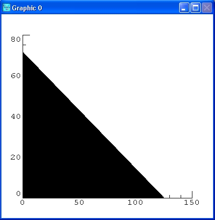
Next we graph the regions specified by the constraints. The last two say that we only need to consider the first quadrant in the x-y plane. Here's a graph delineating the triangular region in the first quadrant determined by the first inequality.
Now let's put in the other two constraint inequalities.
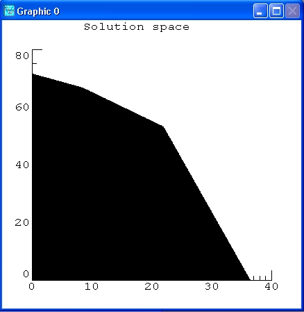
The black area is the solution space that holds valid solutions. This means that any point in this area fulfils the constraints.
Now let's superimpose on top of this picture a contour plot of the objective function P.
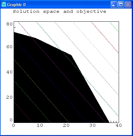
The lines give a picture of the objective function. All solutions that intersect with the black area are valid solutions, meaning that this result also fulfils the set constraints. The more the lines go to the right, the higher the objective value is. The optimal solution or best objective is a line that is still in the black area, but with an as large as possible value.
It seems apparent that the maximum value of P will occur on the level curve (that is, level
line) that passes through the vertex of the polygon that lies near (22,53).
It is the intersection of x + y = 75 and 110*x + 30*y = 4000
This is a corner point of the diagram. This is not a coincidence. The simplex algorithm, which is used
by lpsolve, starts from a theorem that the optimal solution is such a corner point.
In fact we can compute the result:
>>> from numpy import *
>>> from numpy.linalg import inv
>>> x = dot(inv(array([[1, 1], [110, 30]])), array([75, 4000]))
>>> print x
[ 21.875  53.125]
The acreage that results in the maximum profit is 21.875 for wheat and 53.125 for barley. In that case the profit is:
>>> P = dot(array([143, 60]), x)
>>> print P
6315.625
That is, $6315.625.
Note that these command are in script example3.py
Now, lp_solve comes into the picture to solve this linear programming problem more generally. After that we will use it to solve two more complicated problems involving more variables and constraints.
For this example, we use the higher-level script lp_maker to build the model and then some lp_solve API calls to retrieve the solution. Here is again the usage of lp_maker:
 LP_MAKER  Makes mixed integer linear programming problems.

   SYNOPSIS: lp_handle = lp_maker(f,a,b,e,vlb,vub,xint,scalemode,setminim)
      make the MILP problem
        max v = f'*x
          a*x <> b
            vlb <= x <= vub
            x(int) are integer

   ARGUMENTS: The first four arguments are required:
            f: n vector of coefficients for a linear objective function.
            a: m by n matrix representing linear constraints.
            b: m vector of right sides for the inequality constraints.
            e: m vector that determines the sense of the inequalities:
                      e(i) < 0  ==> Less Than
                      e(i) = 0  ==> Equals
                      e(i) > 0  ==> Greater Than
          vlb: n vector of non-negative lower bounds. If empty or omitted,
               then the lower bounds are set to zero.
          vub: n vector of upper bounds. May be omitted or empty.
         xint: vector of integer variables. May be omitted or empty.
    scalemode: Autoscale flag. Off when 0 or omitted.
     setminim: Set maximum lp when this flag equals 0 or omitted.

   OUTPUT: lp_handle is an integer handle to the lp created.
Now let's formulate this model with lp_solve:
>>> from lp_maker import *
>>> f = [143, 60]
>>> A = [[120, 210], [110, 30], [1, 1]]
>>> b = [15000, 4000, 75]
>>> lp = lp_maker(f, A, b, [-1, -1, -1], None, None, None, 1, 0)
>>> solvestat = lpsolve('solve', lp)
>>> obj = lpsolve('get_objective', lp)
>>> print obj
6315.625
>>> x = lpsolve('get_variables', lp)[0]
>>> print x
[21.874999999999993, 53.125000000000007]
>>> lpsolve('delete_lp', lp)
Note that these command are in script example4.py
With the higher-level script lp_maker, we provide all data to lp_solve. lp_solve returns a handle (lp) to the created model. Then the API call 'solve' is used to calculate the optimal solution of the model. The value of the objective function is retrieved via the API call 'get_objective' and the values of the variables are retrieved via the API call 'get_variables'. At last, the model is removed from memory via a call to 'delete_lp'. Don't forget this to free all memory allocated by lp_solve.
The solution is the same answer we obtained before.Ā Note that the non-negativity constraints are accounted implicitly because variables are by default non-negative in lp_solve.
Well, we could have done this problem by hand (as shown in the introduction) because it is very small and it
can be graphically presented.
Now suppose that the farmer is dealing with a third crop, say corn, and that the corresponding data is:
cost per acre $150.75 yield per acre 125 bushels profit per bushel $1.56
With three variables it is already a lot more difficult to show this model graphically. Adding more variables makes it even impossible because we can't imagine anymore how to represent this. We only have a practical understanding of 3 dimensions, but beyond that it is all very theoretical.
If we denote the number of acres allotted to corn by z, then the objective function becomes:
P = (110)(1.30)x + (30)(2.00)yĀ+ (125)(1.56) = 143x + 60y + 195z
And the constraint inequalities are:
120x + 210y + 150.75z <= 15000
110x + 30y + 125z <= 4000
x + y + z <= 75
x >= 0,Āy >= 0, z >= 0
The problem is solved with lp_solve as follows:
>>> from lp_maker import *
>>> f = [143, 60, 195]
>>> A = [[120, 210, 150.75], [110, 30, 125], [1, 1, 1]]
>>> b = [15000, 4000, 75]
>>> lp = lp_maker(f, A, b, [-1, -1, -1], None, None, None, 1, 0)
>>> solvestat = lpsolve('solve', lp)
>>> obj = lpsolve('get_objective', lp)
>>> print obj
6986.84210526
>>> x = lpsolve('get_variables', lp)[0]
>>> print x
[0.0, 56.578947368421055, 18.421052631578945]
>>> lpsolve('delete_lp', lp)
Note that these command are in script example5.py
So the farmer should ditch the wheat and plant 56.5789 acres of barley and 18.4211 acres of corn.
There is no practical limit on the number of variables and constraints that Python can handle. Certainly none that the relatively unsophisticated user will encounter.ĀIndeed, in many true applications of the technique of linear programming, one needs to deal with many variables and constraints.ĀThe solution of such a problem by hand is not feasible, and software like Python is crucial to success.ĀFor example, in the farming problem with which we have been working, one could have more crops than two or three. Think agribusiness instead of family farmer.ĀAnd one could have constraints that arise from other things beside expenses, storage and acreage limitations. For example:
Below is a sequence of commands that solves exactly such a problem. You should be able to recognize the objective expression and the constraints from the data that is entered.Ā But as an aid, you might answer the following questions:
>>> from lpsolve55 import *
>>> from lp_maker import *
>>> f = [110*1.3, 30*2.0, 125*1.56, 75*1.8, 95*.95, 100*2.25, 50*1.35]
>>> A = [[120, 210, 150.75, 115, 186, 140, 85], [110, 30, 125, 75, 95, 100, 50], [1, 1, 1, 1, 1, 1, 1],
         [1, -1, 0, 0, 0, 0, 0], [0, 0, 1, 0, -2, 0, 0], [0, 0, 0, -1, 0, -1, 1]]
>>> b = [55000, 40000, 400, 0, 0, 0]
>>> lp = lp_maker(f, A, b, [-1, -1, -1, -1, -1, -1], [10, 10, 10, 10, 20, 20, 20],
                           [100, Infinite, 50, Infinite, Infinite, 250, Infinite], None, 1, 0)
>>> solvestat = lpsolve('solve', lp)
>>> obj = lpsolve('get_objective', lp)
>>> print obj
75398.0434783
>>> x = lpsolve('get_variables', lp)[0]
>>> print x
[10.0, 10.0, 40.0, 45.652173913043455, 20.0, 250.0, 20.0]
>>> lpsolve('delete_lp', lp)
Note that these command are in script example6.py
Note that we have used in this formulation the vlb and vub arguments of lp_maker. This to set lower and upper bounds on variables. This could have been done via extra constraints, but it is more performant to set bounds on variables. Also note that Infinity is used for variables that have no upper limit.
Note that despite the complexity of the problem, lp_solve solves it almost instantaneously. It seems the farmer should bet the farm on crop number 6.ĀWe strongly suggest you alter the expense and/or the storage limit in the problem and see what effect that has on the answer.
Suppose we want to solve the following linear program using Python:
max 4x1 + 2x2 + x3
s. t. 2x1 + x2 <= 1
x1 + 2x3 <= 2
x1 + x2 + x3 = 1
x1 >= 0
x1 <= 1
x2 >= 0
x2 <= 1
x3 >= 0
x3 <= 2
Convert the LP into Python format we get:
f = [4, 2, 1]
A = [[2, 1, 0], [1, 0, 2], [1, 1, 1]]
b = [1, 2, 1]
Note that constraints on single variables are not put in the constraint matrix. lp_solve can set bounds on individual variables and this is more performant than creating additional constraints. These bounds are:
l = [ 0, 0, 0]
u = [ 1, 1, 2]
Now lets enter this in Python:
>>> f = [4, 2, 1]
>>> A = [[2, 1, 0], [1, 0, 2], [1, 1, 1]]
>>> b = [1, 2, 1]
>>> l = [ 0, 0, 0]
>>> u = [ 1, 1, 2]
Now solve the linear program using Python: Type the commands
>>> from lpsolve55 import *
>>> from lp_maker import *
>>> lp = lp_maker(f, A, b, [-1, -1, -1], l, u, None, 1, 0)
>>> solvestat = lpsolve('solve', lp)
>>> obj = lpsolve('get_objective', lp)
>>> print obj
2.5
>>> x = lpsolve('get_variables', lp)[0]
>>> print x
[0.5, 0.0, 0.5]
>>> lpsolve('delete_lp', lp)
What to do when some of the variables are missing ?
For example, suppose there are no lower bounds on the variables. In this case define l to be the empty set using the Python command:
>>> l = None
This has the same effect as before, because lp_solve has as default lower bound for variables 0.
But what if you want that variables may also become negative?
Then you can use -Infinite as lower bounds:
>>> l = [-Infinite, -Infinite, -Infinite]
Solve this and you get a different result:
>>> lp = lp_maker(f, A, b, [-1, -1, -1], l, u, None, 1, 0)
>>> solvestat = lpsolve('solve', lp)
>>> obj = lpsolve('get_objective', lp)
>>> print obj
2.66666666667
>>> x = lpsolve('get_variables', lp)[0]
>>> print x
[0.66666666666666674, -0.33333333333333348, 0.66666666666666674]
>>> lpsolve('delete_lp', lp)
Note that everwhere where lp is used as argument that this can be a handle (lp) or the models name.
These routines are not part of the lpsolve API, but are added for backwards compatibility. Most of them exist in the lpsolve API with another name.
The lpsolve Python driver is called lpsolve55.pyd (windows) and lpsolve55.so (Unix).
This driver is an interface to the lpsolve55.dll (windows) and liblpsolve55.so (Unix) lpsolve shared library that contains the implementation of lp_solve.
lpsolve55.dll/liblpsolve55.so is distributed with the lp_solve package (archive lp_solve_5.5.2.5_dev.zip/lp_solve_5.5.2.5_dev.tar.gz). The lpsolve Python driver is just
a wrapper between Python and lp_solve to translate the input/output to/from Python and the lp_solve library.
The lpsolve Python driver is written in C. To compile this code a C compiler is needed. Under Unix, this is the standard C compiler (cc/gcc) and under windows it is the Microsoft compiler from Visual Studio .NET. or the mingw gcc compiler This compiler must be called from Python. To make the compilation process easier, a Python script can be used: setup.py (setup64.py for 64 bit OS)
To be able to compile this driver, Python must be installed on the system and callable from a shell or command prompt by just entering the command Python. If this is not the case, set the PATH environment variable to the location where Python is installed. For example C:\Python25
The lpsolve Python driver can use the Python numpy package. To be able to compile the lpsolve driver, this numpy package should also be installed on the system. If the numpy package cannot be found at compilation time, the lpsolve Python driver will not be able to work with numpy. The compilation script setup.py/setup64.py automatically detects if numpy is installed and uses it if found. This is done by searching the numpy directory. This is done by the following python commands:
import sys
import os
p = sys.prefix
NUMPYPATH = ''
if os.path.isdir(p + '/include/numpy'):
  NUMPY = 'NUMPY'
elif os.path.isdir(p + '/Lib/site-packages/numpy/core/include/numpy'):
  NUMPY = 'NUMPY'
  NUMPYPATH = p + '/Lib/site-packages/numpy/core/include'
else:
  NUMPY = 'NONUMPY'
Under Unix, make sure you have enough rights. Possibly you must be logged in as a root user.
Under Windows, the Microsoft visual C compiler is needed by default.
Unfortunately apparently there is a test that the version must be exactly the same as the one where Python itself is build with.
However it is also possible to compile
with the mingw gcc compiler. For this, create (or edit) the file C:\Python25\Lib\distutils\distutils.cfg:
[build]
compiler=mingw32
The python folder can of course be different.
Note that liblpsolve55.a may not exist in directory ../../lpsolve55/bin/win32. Delete it or temporary rename it such that lpsolve55.dll is used.
Now to compile and install the package, just enter the following in a command prompt/shell:
python setup.py installor
python setup64.py install
and everything is done.
To create a distribution package, enter:
python setup.py bdist
Under Windows, use:
python setup.py bdist_wininst
Under Linux, the distributable packages is called lpsolve55-5.5.0.6.linux-i686.tar.gz
The contents must be expanded to the appropriate directory.
Under Windows, there is an installer that installs the Python lpsolve driver and the supporting scripts lp_maker.py and lp_solve.py. Just run lpsolve55-5.5.0.6.win32-py2.4.exe (this installer is in archive lp_solve_5.5_Python_exe.zip).
On other platforms, the lpsolve driver must be compiled as described in the previous section: Compile the lpsolve driver
Don't forget that lpsolve55.dll (Windows) or liblpsolve55.so (Unix/Linux) is also needed for this (In archive lp_solve_5.5.2.5_dev.zip).
See also Using lpsolve from MATLAB, Using lpsolve from O-Matrix, Using lpsolve from Sysquake, Using lpsolve from Scilab, Using lpsolve from Octave, Using lpsolve from FreeMat, Using lpsolve from Euler, Using lpsolve from PHP, Using lpsolve from Sage, Using lpsolve from R, Using lpsolve from Microsoft Solver Foundation