GNU Octave is a high-level language, primarily intended for numerical computations. It provides a convenient command line interface for solving linear and non-linear problems numerically, and for performing other numerical experiments. It may also be used as a batch-oriented language.
GNU Octave is also freely redistributable software.
We will not discuss the specifics of Octave here but instead refer the reader to the Octave website and GNU Octave Repository.
lpsolve is callable from Octave via a dynamic linked function. As such, it looks like lpsolve is fully integrated with Octave. Matrices can directly be transferred between Octave and lpsolve in both directions. The complete interface is written in C so it has maximum performance. The whole lpsolve API is implemented with some extra's specific for Octave (especially for matrix support). So you have full control to the complete lpsolve functionality via the octlpsolve Octave driver. If you find that this involves too much work to solve an lp model then you can also work via higher-level script files that can make things a lot easier. See further in this article.
Note that your version of Octave must support dynamic linking. To find out if it does, type the command:
octave_config_info ("ENABLE_DYNAMIC_LINKING")
at the Octave prompt. Support for dynamic linking is included if this expression returns the string "true".
If this is not the case, then Octave is not able to call dynamic linked routines and as such also not lpsolve. In that case you must recompile Octave with dynamic linked routines enabled. Under Linux, the following commands must be executed for this:
configure --enable-shared
make
See Installing Octave for more information.
Under Windows, dynamic linking should already be active. If not, then Octave must be recompiled. The following document can help in this process: README.Windows
The octave dynamic linked routine is in a file with extension .oct. It is impossible to provide a precompiled octlpsolve.oct file with the lpsolve distribution because the structure of the .oct files change often on new releases of Octave and are not compatible with each other. Therefore you must build the driver yourself. Look at the end of this document how to do this.
A driver program is needed: octlpsolve (octlpsolve.oct). This driver must be put in a directory known to Octave (in one of the directories from the Octave 'path' command) and Octave can call the octlpsolve solver.
This driver calls lpsolve via the lpsolve shared library (lpsolve55.dll under Windows and liblpsolve55.so under Unix/Linux) (in archives lp_solve_5.5.2.0_dev.zip/lp_solve_5.5.2.0_dev.tar.gz). This has the advantage that the octlpsolve driver doesn't have to be recompiled when an update of lpsolve is provided.
So note the difference between the Octave lpsolve driver that is called octlpsolve and the lpsolve library that implements the API that is called lpsolve55.
There are also some Octave script files (.m) as a quick start.
To test if everything is installed correctly, enter octlpsolve in the Octave command window. If it gives the following, then everything is ok:
octlpsolve  Octave Interface version 5.5.0.6
using lpsolve version 5.5.2.0

Usage: [ret1, ret2, ...] = octlpsolve('functionname', arg1, arg2, ...)
However, if you get the following:
error: 'octlpsolve' undefined near line 2 column 1
Then Octave cannot find octlpsolve.oct
If you get the following:
error: Failed to initialise lpsolve library.
Then Octave can find the octlpsolve driver program, but the driver program cannot find the lpsolve library that contains the lpsolve implementation. This library is called lpsolve55.dll under Windows and liblpsolve55.so under Unix/Linux. Under Windows, the dll should be in a directory specified by the PATH environment variables and under Unix/Linux in directory /lib, /usr/lib or a directory defined by LD_LIBRARY_PATH.
In the following text, octave:> before the Octave commands is the Octave prompt. Only the text after octave:> must be entered. Note that the default prompt also contains an incrementing number starting from one each time Octave starts. For this documentation, the default Octave was changed with the following command: PS1 = "\\s:> "
To call an lpsolve function, the following syntax must be used:
octave:> [ret1, ret2, ...] = octlpsolve('functionname', arg1, arg2, ...)
The return values are optional and depend on the function called. functionname must always be enclosed between single or double quotes to make it alphanumerical and it is case sensitive. The number and type of arguments depend on the function called. Some functions even have a variable number of arguments and a different behaviour occurs depending on the type of the argument. functionname can be (almost) any of the lpsolve API routines (see lp_solve API reference) plus some extra Octave specific functions. Most of the lpsolve API routines use or return an lprec structure. To make things more robust in Octave, this structure is replaced by a handle or the model name. The lprec structures are maintained internally by the lpsolve driver. The handle is an incrementing number starting from 0. Starting from driver version 5.5.0.2, it is also possible to use the model name instead of the handle. This can of course only be done if a name is given to the model. This is done via lpsolve routine set_lp_name or by specifying the model name in routine read_lp. See Using model name instead of handle.
Almost all callable functions can be found in the lp_solve API reference. Some are exactly as described in the reference guide, others have a slightly different syntax to make maximum use of the Octave functionality. For example make_lp is used identical as described. But get_variables is slightly different. In the API reference, this function has two arguments. The first the lp handle and the second the resulting variables and this array must already be dimensioned. When lpsolve is used from Octave, nothing must be dimensioned in advance. The octlpsolve driver takes care of dimensioning all return variables and they are always returned as return value of the call to octlpsolve. Never as argument to the routine. This can be a single value as for get_objective (although Octave stores this in a 1x1 matrix) or a matrix or vector as in get_variables. In this case, get_variables returns a 4x1 matrix (vector) with the result of the 4 variables of the lp model.
Note that you can get an overview of the available functionnames and their arguments by entering the following in Octave:
>> help octlpsolve.m
(Note that you can execute this example by entering command per command as shown below or by just entering example1. This will execute example1.m. You can see its contents by entering type example1.m)
octave:> lp=octlpsolve('make_lp', 0, 4);
octave:> octlpsolve('set_verbose', lp, 3);
octave:> octlpsolve('set_obj_fn', lp, [1, 3, 6.24, 0.1]);
octave:> octlpsolve('add_constraint', lp, [0, 78.26, 0, 2.9], 2, 92.3);
octave:> octlpsolve('add_constraint', lp, [0.24, 0, 11.31, 0], 1, 14.8);
octave:> octlpsolve('add_constraint', lp, [12.68, 0, 0.08, 0.9], 2, 4);
octave:> octlpsolve('set_lowbo', lp, 1, 28.6);
octave:> octlpsolve('set_lowbo', lp, 4, 18);
octave:> octlpsolve('set_upbo', lp, 4, 48.98);
octave:> octlpsolve('set_col_name', lp, 1, 'COLONE');
octave:> octlpsolve('set_col_name', lp, 2, 'COLTWO');
octave:> octlpsolve('set_col_name', lp, 3, 'COLTHREE');
octave:> octlpsolve('set_col_name', lp, 4, 'COLFOUR');
octave:> octlpsolve('set_row_name', lp, 1, 'THISROW');
octave:> octlpsolve('set_row_name', lp, 2, 'THATROW');
octave:> octlpsolve('set_row_name', lp, 3, 'LASTROW');
octave:> octlpsolve('write_lp', lp, 'a.lp');
octave:> octlpsolve('get_mat', lp, 1, 2)
ans = 78.260
octave:> octlpsolve('solve', lp)
ans = 0
octave:> octlpsolve('get_objective', lp)
ans = 31.783
octave:> octlpsolve('get_variables', lp)
ans =

  28.60000
   0.00000
   0.00000
  31.82759

octave:> octlpsolve('get_constraints', lp)
ans =

   92.3000
    6.8640
  391.2928
Note that there are some commands that return an answer. To see the answer, the command was not terminated with a semicolon (;). If the semicolon is put at the end of a command, the answer is not shown. However it is also possible to write the answer in a variable. For example:
octave:> obj=octlpsolve('get_objective', lp)
obj = 31.783
Or without echoing on screen:
octave:> obj=octlpsolve('get_objective', lp);
The last command will only write the result in variable obj without showing anything on screen. get_variables and get_constraints return a vector with the result. This can also be put in a variable:
octave:> x=octlpsolve('get_variables', lp);
octave:> b=octlpsolve('get_constraints', lp);
It is always possible to show the contents of a variable by just giving it as command:
octave:> x
x =

  28.60000
   0.00000
   0.00000
  31.82759
Don't forget to free the handle and its associated memory when you are done:
octave:> octlpsolve('delete_lp', lp);
octave:> lp=octlpsolve('make_lp', 0, 4);
octave:> octlpsolve('set_lp_name', lp, 'mymodel');
octave:> octlpsolve('set_verbose', 'mymodel', 3);
octave:> octlpsolve('set_obj_fn', 'mymodel', [1, 3, 6.24, 0.1]);
octave:> octlpsolve('add_constraint', 'mymodel', [0, 78.26, 0, 2.9], 2, 92.3);
octave:> octlpsolve('add_constraint', 'mymodel', [0.24, 0, 11.31, 0], 1, 14.8);
octave:> octlpsolve('add_constraint', 'mymodel', [12.68, 0, 0.08, 0.9], 2, 4);
octave:> octlpsolve('set_lowbo', 'mymodel', 1, 28.6);
octave:> octlpsolve('set_lowbo', 'mymodel', 4, 18);
octave:> octlpsolve('set_upbo', 'mymodel', 4, 48.98);
octave:> octlpsolve('set_col_name', 'mymodel', 1, 'COLONE');
octave:> octlpsolve('set_col_name', 'mymodel', 2, 'COLTWO');
octave:> octlpsolve('set_col_name', 'mymodel', 3, 'COLTHREE');
octave:> octlpsolve('set_col_name', 'mymodel', 4, 'COLFOUR');
octave:> octlpsolve('set_row_name', 'mymodel', 1, 'THISROW');
octave:> octlpsolve('set_row_name', 'mymodel', 2, 'THATROW');
octave:> octlpsolve('set_row_name', 'mymodel', 3, 'LASTROW');
octave:> octlpsolve('write_lp', 'mymodel', 'a.lp');
octave:> octlpsolve('get_mat', 'mymodel', 1, 2)
ans = 78.260
octave:> octlpsolve('solve', 'mymodel')
ans = 0
octave:> octlpsolve('get_objective', 'mymodel')
ans = 31.783
octave:> octlpsolve('get_variables', 'mymodel')
ans =

  28.60000
   0.00000
   0.00000
  31.82759

octave:> octlpsolve('get_constraints', 'mymodel')
ans =

   92.3000
    6.8640
  391.2928
So everywhere a handle is needed, you can also use the model name. You can even mix the two methods.
There is also a specific Octave routine to get the handle from the model name: get_handle.
For example:
>> octlpsolve('get_handle', 'mymodel')
0
Don't forget to free the handle and its associated memory when you are done:
octave:> octlpsolve('delete_lp', 'mymodel');
In the next part of this documentation, the handle is used. But if you name the model, the name could thus also be used.
octave:> octlpsolve('add_constraint', lp, [0.24, 0, 11.31, 0], 1, 14.8);
Most of the time, variables are used to provide the data:
octave:> octlpsolve('add_constraint', lp, a1, 1, 14.8);
Where a1 is a matrix variable.
Most of the time, octlpsolve needs vectors (rows or columns). In all situations, it doesn't matter if the vectors are row or column vectors. The driver accepts them both. For example:
octave:> octlpsolve('add_constraint', lp, [0.24; 0; 11.31; 0], 1, 14.8);
Which is a column vector, but it is also accepted.
An important final note. Several lp_solve API routines accept a vector where the first element (element 0) is not used. Other lp_solve API calls do use the first element. In the Octave interface, there is never an unused element in the matrices. So if the lp_solve API specifies that the first element is not used, then this element is not in the Octave matrix.
All numerical data is stored in matrices. Alphanumerical data, however, is more difficult to store in matrices. Matrices require that each element has the same size (length) and that is difficult and unpractical for alphanumerical data. In a limited number of lpsolve routines, alphanumerical data is required or returned and in some also multiple elements. An example is set_col_name. For this, Octave sets are used. To specify a set of alphanumerical elements, the following notation is used: { 'element1', 'element2', ... }. Note the { and } symbols instead of [ and ] that are used with matrices.
Because Octave is all about matrices, all lpsolve API routines that need a column or row number to get/set information for that
column/row are extended in the octlpsolve Octave driver to also work with matrices. For example set_int in the API can
only set the integer status for one column. If the status for several integer variables must be set, then set_int
must be called multiple times. The octlpsolve Octave driver however also allows specifying a vector to set the integer
status of all variables at once. The API call is: return = octlpsolve('set_int', lp, column, must_be_int). The
matrix version of this call is: return = octlpsolve('set_int', lp, [must_be_int]).
The API call to return the integer status of a variable is: return = octlpsolve('is_int', lp, column). The
matrix version of this call is: [is_int] = octlpsolve('is_int', lp)
Also note the get_mat and set_mat routines. In Octave these are extended to return/set the complete constraint matrix.
See following example.
Above example can thus also be done as follows:
(Note that you can execute this example by entering command per command as shown below or by just entering example2.
This will execute example2.m. You can see its contents by entering type example2.m)
octave:> lp=octlpsolve('make_lp', 0, 4);
octave:> octlpsolve('set_verbose', lp, 3);
octave:> octlpsolve('set_obj_fn', lp, [1, 3, 6.24, 0.1]);
octave:> octlpsolve('add_constraint', lp, [0, 78.26, 0, 2.9], 2, 92.3);
octave:> octlpsolve('add_constraint', lp, [0.24, 0, 11.31, 0], 1, 14.8);
octave:> octlpsolve('add_constraint', lp, [12.68, 0, 0.08, 0.9], 2, 4);
octave:> octlpsolve('set_lowbo', lp, [28.6, 0, 0, 18]);
octave:> octlpsolve('set_upbo', lp, [Inf, Inf, Inf, 48.98]);
octave:> octlpsolve('set_col_name', lp, {'COLONE', 'COLTWO', 'COLTHREE', 'COLFOUR'});
octave:> octlpsolve('set_row_name', lp, {'THISROW', 'THATROW', 'LASTROW'});
octave:> octlpsolve('write_lp', lp, 'a.lp');
octave:> octlpsolve('get_mat', lp)
ans =

   0.00000  78.26000   0.00000   2.90000
   0.24000   0.00000  11.31000   0.00000
  12.68000   0.00000   0.08000   0.90000

octave:> octlpsolve('solve', lp)
ans = 0
octave:> octlpsolve('get_objective', lp)
ans = 31.783
octave:> octlpsolve('get_variables', lp)
ans =

  28.60000
   0.00000
   0.00000
  31.82759

octave:> octlpsolve('get_constraints', lp)
ans =

   92.3000
    6.8640
  391.2928
Note the usage of Inf in set_upbo. This stands for 'infinity'. Meaning an infinite upper bound. It is also possible to use -Inf to express minus infinity. This can for example be used to create a free variable.
To show the full power of the matrices, let's now do some matrix calculations to check the solution. It works further on above example:
octave:> A=octlpsolve('get_mat', lp);
octave:> X=octlpsolve('get_variables', lp);
octave:> B = A * X
B =

   92.3000
    6.8640
  391.2928
So what we have done here is calculate the values of the constraints (RHS) by multiplying the constraint matrix with the solution vector. Now take a look at the values of the constraints that lpsolve has found:
octave:> octlpsolve('get_constraints', lp)
ans =

   92.3000
    6.8640
  391.2928
Exactly the same as the calculated B vector, as expected.
Also the value of the objective can be calculated in a same way:
octave:> C=octlpsolve('get_obj_fn', lp);
octave:> X=octlpsolve('get_variables', lp);
octave:> obj = C * X
obj = 31.783
So what we have done here is calculate the value of the objective by multiplying the objective vector with the solution vector. Now take a look at the value of the objective that lpsolve has found:
octave:> octlpsolve('get_objective', lp)
ans = 31.783
Again exactly the same as the calculated obj value, as expected.
octave:> lp=octlpsolve('make_lp', 0, 4);
octave:> octlpsolve('set_verbose', lp, 3);
octave:> octlpsolve('add_constraint', lp, [0, 78.26, 0, 2.9], 2, 92.3);
octave:> octlpsolve('add_constraint', lp, [0.24, 0, 11.31, 0], 1, 14.8);
octave:> octlpsolve('add_constraint', lp, [12.68, 0, 0.08, 0.9], 2, 4);
Note the 3rd parameter on set_verbose and the 4th on add_constraint. These are lp_solve constants. One could define all the possible constants in Octave and then use them in the calls, but that has several disadvantages. First there stays the possibility to provide a constant that is not intended for that particular call. Another issue is that calls that return a constant are still returning it numerical.
Both issues can now be handled by string constants. The above code can be done as following with string constants:
octave:> lp=octlpsolve('make_lp', 0, 4);
octave:> octlpsolve('set_verbose', lp, 'IMPORTANT');
octave:> octlpsolve('add_constraint', lp, [0, 78.26, 0, 2.9], 'GE', 92.3);
octave:> octlpsolve('add_constraint', lp, [0.24, 0, 11.31, 0], 'LE', 14.8);
octave:> octlpsolve('add_constraint', lp, [12.68, 0, 0.08, 0.9], 'GE', 4);
This is not only more readable, there is much lesser chance that mistakes are being made. The calling routine knows which constants are possible and only allows these. So unknown constants or constants that are intended for other calls are not accepted. For example:
octave:> octlpsolve('set_verbose', lp, 'blabla');
error: BLABLA: Unknown.

octave:> octlpsolve('set_verbose', lp, 'GE');
error: GE: Not allowed here.
Note the difference between the two error messages. The first says that the constant is not known, the second that the constant cannot be used at that place.
Constants are case insensitive. Internally they are always translated to upper case. Also when returned they will always be in upper case.
The constant names are the ones as specified in the documentation of each API routine. There are only 3 exceptions, extensions actually. 'LE', 'GE' and 'EQ' in add_constraint and is_constr_type can also be '<', '<=', '>', '>=', '='. When returned however, 'GE', 'LE', 'EQ' will be used.
Also in the matrix version of calls, string constants are possible. For example:
octave:> octlpsolve('set_constr_type', lp, {'LE', 'EQ', 'GE'});
Some constants can be a combination of multiple constants. For example set_scaling:
octave:> octlpsolve('set_scaling', lp, 3+128);
With the string version of constants this can be done as following:
octave:> octlpsolve('set_scaling', lp, 'SCALE_MEAN|SCALE_INTEGERS');
| is the OR operator used to combine multiple constants. There may optinally be spaces before and after the |.
Not all OR combinations are legal. For example in set_scaling, a choice must be made between SCALE_EXTREME, SCALE_RANGE, SCALE_MEAN, SCALE_GEOMETRIC or SCALE_CURTISREID. They may not be combined with each other. This is also tested:
octave:> octlpsolve('set_scaling', lp, 'SCALE_MEAN|SCALE_RANGE');
error: SCALE_RANGE cannot be combined with SCALE_MEAN
Everywhere constants must be provided, numeric or string values may be provided. The routine automatically interpretes them.
Returning constants is a different story. The user must let lp_solve know how to return it. Numerical or as string. The default is numerical:
octave:> octlpsolve('get_scaling', lp)
ans = 131
To let lp_solve return a constant as string, a call to a new function must be made: return_constants
octave:> octlpsolve('return_constants', 1);
From now on, all returned constants are returned as string:
octave:> octlpsolve('get_scaling', lp)
ans = SCALE_MEAN|SCALE_INTEGERS
Also when an array of constants is returned, they are returned as string when return_constants is set:
octave:> octlpsolve('get_constr_type', lp)
ans =
{
  [1,1] = LE
  [1,2] = EQ
  [1,3] = GE
}
This for all routines until return_constants is again called with 0:
octave:> octlpsolve('return_constants', 0);
The (new) current setting of return_constants is always returned by the call. Even when set:
octave:> octlpsolve('return_constants', 1)
ans = 1
To get the value without setting it, don't provide the second argument:
octave:> octlpsolve('return_constants')
ans = 1
In the next part of this documentation, return_constants is the default, 0, so all constants are returned numerical and provided constants are also numerical. This to keep the documentation as compatible as possible with older versions. But don't let you hold that back to use string constants in your code.
Octave can execute a sequence of statements stored in diskfiles. Script files mostly have the file type of ".m" as the last part of their filename (extension). Much of your work with Octave will be in creating and refining script files. Script files are usually created using your local editor.
Script files can be compared with batch files or scripts. You can put Octave commands in them and execute them at any time. The script file is executed like any other command, by entering its name (without the .m extension).
The octlpsolve Octave distribution contains some example script files to demonstrate this.
To see the contents of such a file, enter the command 'type filename'. You can also edit these files with your favourite text editor (or notepad).
Contains the commands as shown in the first example of this article.
Contains the commands as shown in the second example of this article.
Contains the commands of a practical example. See further in this article.
Contains the commands of a practical example. See further in this article.
Contains the commands of a practical example. See further in this article.
This script uses the API to create a higher-level function called lp_solve. This function accepts as arguments some matrices and options to create and solve an lp model. See the beginning of the file or type help lp_solve or just lp_solve to see its usage:
 LP_SOLVE  Solves mixed integer linear programming problems.

   SYNOPSIS: [obj,x,duals] = lp_solve(f,a,b,e,vlb,vub,xint,scalemode,keep)

      solves the MILP problem

              max v = f'*x
                a*x <> b
                  vlb <= x <= vub
                  x(int) are integer

   ARGUMENTS: The first four arguments are required:

            f: n vector of coefficients for a linear objective function.
            a: m by n matrix representing linear constraints.
            b: m vector of right sides for the inequality constraints.
            e: m vector that determines the sense of the inequalities:
                      e(i) = -1  ==> Less Than
                      e(i) =  0  ==> Equals
                      e(i) =  1  ==> Greater Than
          vlb: n vector of lower bounds. If empty or omitted,
               then the lower bounds are set to zero.
          vub: n vector of upper bounds. May be omitted or empty.
         xint: vector of integer variables. May be omitted or empty.
    scalemode: scale flag. Off when 0 or omitted.
         keep: Flag for keeping the lp problem after it's been solved.
               If omitted, the lp will be deleted when solved.

   OUTPUT: A nonempty output is returned if a solution is found:

          obj: Optimal value of the objective function.
            x: Optimal value of the decision variables.
        duals: solution of the dual problem.
Example of usage. To create and solve following lp-model:
max: -x1 + 2 x2;
C1: 2x1 + x2 < 5;
-4 x1 + 4 x2 <5;

int x2,x1;
The following command can be used:
octave:> [obj, x]=lp_solve([-1, 2], [2, 1; -4, 4], [5, 5], [-1, -1], [], [], [1, 2])
obj = 3
x =

  1
  2
This script is analog to the lp_solve script and also uses the API to create a higher-level function called lp_maker. This function accepts as arguments some matrices and options to create an lp model. Note that this scripts only creates a model and returns a handle. See the beginning of the file or type help lp_maker or just lp_maker to see its usage:
octave:> help lp_maker

 LP_MAKER  Makes mixed integer linear programming problems.

   SYNOPSIS: lp_handle = lp_maker(f,a,b,e,vlb,vub,xint,scalemode,setminim)
      make the MILP problem
        max v = f'*x
          a*x <> b
            x >= vlb >= 0
            x <= vub
            x(int) are integer

   ARGUMENTS: The first four arguments are required:
            f: n vector of coefficients for a linear objective function.
            a: m by n matrix representing linear constraints.
            b: m vector of right sides for the inequality constraints.
            e: m vector that determines the sense of the inequalities:
                      e(i) < 0  ==> Less Than
                      e(i) = 0  ==> Equals
                      e(i) > 0  ==> Greater Than
          vlb: n vector of non-negative lower bounds. If empty or omitted,
               then the lower bounds are set to zero.
          vub: n vector of upper bounds. May be omitted or empty.
         xint: vector of integer variables. May be omitted or empty.
    scalemode: scale flag. Off when 0 or omitted.
     setminim: Set maximum lp when this flag equals 0 or omitted.

   OUTPUT: lp_handle is an integer handle to the lp created.
Example of usage. To create following lp-model:
max: -x1 + 2 x2;
C1: 2x1 + x2 < 5;
-4 x1 + 4 x2 <5;

int x2,x1;
The following command can be used:
octave:> lp=lp_maker([-1, 2], [2, 1; -4, 4], [5, 5], [-1, -1], [], [], [1, 2])
lp = 0
To solve the model and get the solution:
octave:> octlpsolve('solve', lp)
ans = 0

octave:> octlpsolve('get_objective', lp)
ans = 3

octave:> octlpsolve('get_variables', lp)
ans =

  1
  2
Don't forget to free the handle and its associated memory when you are done:
octave:> octlpsolve('delete_lp', lp);
Contains several examples to build and solve lp models.
Contains several examples to build and solve lp models. Also solves the lp_examples from the lp_solve distribution.
We shall illustrate the method of linear programming by means of a simple example, giving a combination graphical/numerical solution, and then solve both a slightly as well as a substantially more complicated problem.
Suppose a farmer has 75 acres on which to plant two crops: wheat and barley. To produce these crops, it costs the farmer (for seed, fertilizer, etc.) $120 per acre for the wheat and� $210 per acre for the barley.�The farmer has $15000 available for expenses. But after the harvest, the farmer must store the crops while awaiting favourable market conditions. The farmer has storage space for 4000 bushels.�Each acre yields an average of 110 bushels of wheat or 30 bushels of barley.� If the net profit per bushel of wheat (after all expenses have been subtracted) is $1.30 and for barley is $2.00, how should the farmer plant the 75 acres to maximize profit?
We begin by formulating the problem mathematically.� First we express the objective, that is the profit, and the constraints algebraically, then we graph them, and lastly we arrive at the solution by graphical inspection and a minor arithmetic calculation.
Let x denote the number of acres allotted to wheat and y the number of acres allotted to barley. Then the expression to be maximized, that is the profit, is clearly
P = (110)(1.30)x + (30)(2.00)y = 143x + 60y.
There are three constraint inequalities, specified by the limits on expenses, storage and acreage. They are respectively:
120x + 210y <= 15000
110x + 30y <= 4000
x + y <= 75
Strictly speaking there are two more constraint inequalities forced by the fact that the farmer cannot plant a negative number of acres, namely:
x >= 0,�y >= 0.
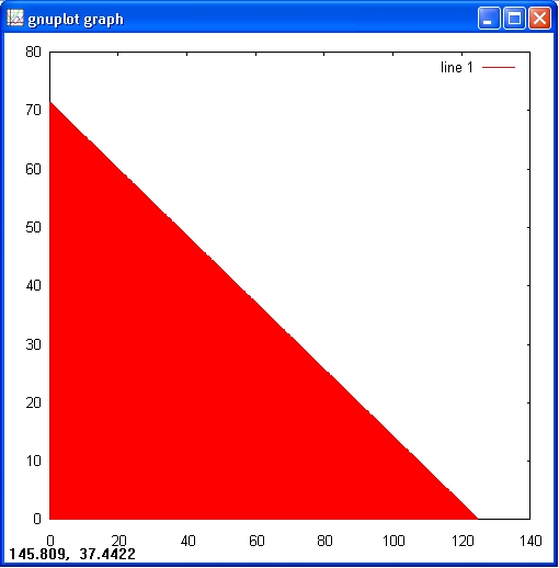
Next we graph the regions specified by the constraints. The last two say that we only need to consider the first quadrant in the x-y plane. Here's a graph delineating the triangular region in the first quadrant determined by the first inequality.
octave:> X = 0.1:0.1:125;
octave:> Y1 = (15000 - 120.*X)./210;
octave:> bar(X, Y1);
Now let's put in the other two constraint inequalities.
octave:> X = 0.1:0.05:40;
octave:> Y1 = (15000. - 120*X)/210;
octave:> Y2 = max((4000 - 110.*X)./30, 0);
octave:> Y3 = max(75 - X, 0);
octave:> Ytop = min([Y1; Y2; Y3]);
octave:> bar(X, Ytop);
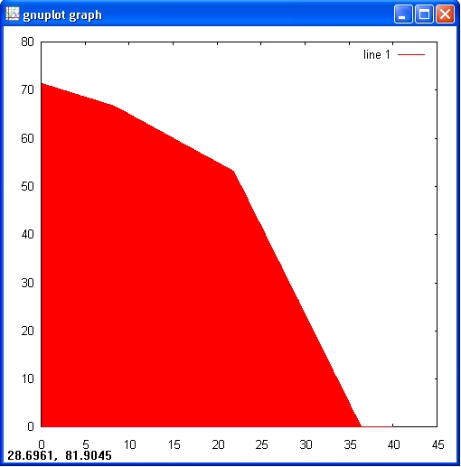
The red area is the solution space that holds valid solutions. This means that any point in this area fulfils the constraints.
Now let's superimpose on top of this picture the objective function P.
octave:> hold on
octave:> X=15:25:40;
octave:> title('Solution space and objective')
octave:> plot(X,(6315.63-143.0*X)/60.0);
octave:> hold off
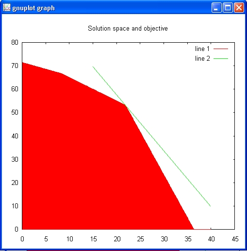
The line gives a picture of the objective function. All solutions that intersect with the red area are valid solutions, meaning that this result also fulfils the set constraints. The more the line goes to the right, the higher the objective value is. The optimal solution or best objective is a line that is still in the red area, but with an as large as possible value.
It seems apparent that the maximum value of P will occur on the level curve (that is, level
line) that passes through the vertex of the polygon that lies near (22,53).
It is the intersection of x + y = 75 and 110*x + 30*y = 4000
This is a corner point of the diagram. This is not a coincidence. The simplex algorithm, which is used
by lp_solve, starts from a theorem that the optimal solution is such a corner point.
In fact we can compute the result:
octave:> x = [1 1; 110 30] \ [75; 4000]
x =

   21.875
   53.125
The acreage that results in the maximum profit is 21.875 for wheat and 53.125 for barley. In that case the profit is:
octave:> P = [143 60] * x
P = 6315.6
That is, $6315.6.
Note that these command are in script example3.m
Now, lp_solve comes into the picture to solve this linear programming problem more generally. After that we will use it to solve two more complicated problems involving more variables and constraints.
For this example, we use the higher-level script lp_maker to build the model and then some lp_solve API calls to retrieve the solution. Here is again the usage of lp_maker:
 LP_MAKER  Makes mixed integer linear programming problems.

   SYNOPSIS: lp_handle = lp_maker(f,a,b,e,vlb,vub,xint,scalemode,setminim)
      make the MILP problem
        max v = f'*x
          a*x <> b
            x >= vlb >= 0
            x <= vub
            x(int) are integer

   ARGUMENTS: The first four arguments are required:
            f: n vector of coefficients for a linear objective function.
            a: m by n matrix representing linear constraints.
            b: m vector of right sides for the inequality constraints.
            e: m vector that determines the sense of the inequalities:
                      e(i) < 0  ==> Less Than
                      e(i) = 0  ==> Equals
                      e(i) > 0  ==> Greater Than
          vlb: n vector of non-negative lower bounds. If empty or omitted,
               then the lower bounds are set to zero.
          vub: n vector of upper bounds. May be omitted or empty.
         xint: vector of integer variables. May be omitted or empty.
    scalemode: scale flag. Off when 0 or omitted.
     setminim: Set maximum lp when this flag equals 0 or omitted.

   OUTPUT: lp_handle is an integer handle to the lp created.
Now let's formulate this model with lp_solve:
octave:> f = [143 60];
octave:> A = [120 210; 110 30; 1 1];
octave:> b = [15000; 4000; 75];
octave:> lp = lp_maker(f, A, b, [-1; -1; -1], [], [], [], 1, 0);
octave:> solvestat = octlpsolve('solve', lp)
solvestat = 0
octave:> obj = octlpsolve('get_objective', lp)
obj = 6315.6
octave:> x = octlpsolve('get_variables', lp)
x =

  21.875
  53.125

octave:> octlpsolve('delete_lp', lp);
Note that these command are in script example4.m
With the higher-level script lp_maker, we provide all data to lp_solve. lp_solve returns a handle (lp) to the created model. Then the API call 'solve' is used to calculate the optimal solution of the model. The value of the objective function is retrieved via the API call 'get_objective' and the values of the variables are retrieved via the API call 'get_variables'. At last, the model is removed from memory via a call to 'delete_lp'. Don't forget this to free all memory allocated by lp_solve.
The solution is the same answer we obtained before.� Note that the non-negativity constraints are accounted implicitly because variables are by default non-negative in lp_solve.
Well, we could have done this problem by hand (as shown in the introduction) because it is very small and it
can be graphically presented.
Now suppose that the farmer is dealing with a third crop, say corn, and that the corresponding data is:
cost per acre $150.75 yield per acre 125 bushels profit per bushel $1.56
With three variables it is already a lot more difficult to show this model graphically. Adding more variables makes it even impossible because we can't imagine anymore how to represent this. We only have a practical understanding of 3 dimentions, but beyound that it is all very theorethical.
If we denote the number of acres allotted to corn by z, then the objective function becomes:
P = (110)(1.30)x + (30)(2.00)y�+ (125)(1.56) = 143x + 60y + 195z
And the constraint inequalities are:
120x + 210y + 150.75z <= 15000
110x + 30y + 125z <= 4000
x + y + z <= 75
x >= 0,�y >= 0, z >= 0
The problem is solved with lp_solve as follows:
octave:> f = [143 60 195];
octave:> A = [120 210 150.75; 110 30 125; 1 1 1];
octave:> b = [15000; 4000; 75];
octave:> lp = lp_maker(f, A, b, [-1; -1; -1], [], [], [], 1, 0);
octave:> solvestat = octlpsolve('solve', lp)
solvestat = 0
octave:> obj = octlpsolve('get_objective', lp)
obj = 6986.8
octave:> x = octlpsolve('get_variables', lp)
x =

   0.00000
  56.57895
  18.42105

octave:> octlpsolve('delete_lp', lp);
Note that these command are in script example5.m
So the farmer should ditch the wheat and plant 56.5789 acres of barley and 18.4211 acres of corn.
There is no practical limit on the number of variables and constraints that Octave can handle. Certainly none that the relatively unsophisticated user will encounter.�Indeed, in many true applications of the technique of linear programming, one needs to deal with many variables and constraints.�The solution of such a problem by hand is not feasible, and software like Octave is crucial to success.�For example, in the farming problem with which we have been working, one could have more crops than two or three. Think agribusiness instead of family farmer.�And one could have constraints that arise from other things beside expenses, storage and acreage limitations. For example:
Below is a sequence of commands that solves exactly such a problem. You should be able to recognize the objective expression and the constraints from the data that is entered.� But as an aid, you might answer the following questions:
octave:> f = [110*1.3 30*2.0 125*1.56 75*1.8 95*.95 100*2.25 50*1.35];
octave:> A = [120 210 150.75 115 186 140 85;
        110 30 125 75 95 100 50;
        1 1 1 1 1 1 1;
        1 -1 0 0 0 0 0;
        0 0 1 0 -2 0 0;
        0 0 0 -1 0 -1 1];

octave:> b = [55000;40000;400;0;0;0];
octave:> lp = lp_maker(f, A, b, [-1; -1; -1; -1; -1; -1],
                          [10 10 10 10 20 20 20], [100 Inf 50 Inf Inf 250 Inf], [], 1, 0);
octave:> solvestat = octlpsolve('solve', lp)
solvestat = 0
octave:> obj = octlpsolve('get_objective', lp)
obj =  7.5398e+04
octave:> x = octlpsolve('get_variables', lp)
x =

   10.000
   10.000
   40.000
   45.652
   20.000
  250.000
   20.000

octave:> octlpsolve('delete_lp', lp);
Note that these command are in script example6.m
Note that we have used in this formulation the vlb and vub arguments of lp_maker. This to set lower and upper bounds on variables. This could have been done via extra constraints, but it is more performant to set bounds on variables. Also note that Inf is used for variables that have no upper limit. This stands for Infinity.
Note that despite the complexity of the problem, lp_solve solves it almost instantaneously. It seems the farmer should bet the farm on crop number 6.�We strongly suggest you alter the expense and/or the storage limit in the problem and see what effect that has on the answer.
Suppose we want to solve the following linear program using Octave:
max 4x1 + 2x2 + x3
s. t. 2x1 + x2 <= 1
x1 + 2x3 <= 2
x1 + x2 + x3 = 1
x1 >= 0
x1 <= 1
x2 >= 0
x2 <= 1
x3 >= 0
x3 <= 2
Convert the LP into Octave format we get:
f = [4 2 1]
A = [2 1 0; 1 0 2; 1 1 1]
b = [1; 2; 1]
Note that constraints on single variables are not put in the constraint matrix. lp_solve can set bounds on individual variables and this is more performant than creating additional constraints. These bounds are:
l = [ 0 0 0]
u = [ 1 1 2]
Now lets enter this in Octave:
octave:> f = [4 2 1];
octave:> A = [2 1 0; 1 0 2; 1 1 1];
octave:> b = [1; 2; 1];
octave:> l = [ 0 0 0];
octave:> u = [ 1 1 2];
Now solve the linear program using Octave: Type the commands
octave:> lp = lp_maker(f, A, b, [-1; -1; -1], l, u, [], 1, 0);
octave:> solvestat = octlpsolve('solve', lp)
solvestat = 0
octave:> obj = octlpsolve('get_objective', lp)
obj = 2.5000
octave:> x = octlpsolve('get_variables', lp)
x =

  0.50000
  0.00000
  0.50000

octave:> octlpsolve('delete_lp', lp)
What to do when some of the variables are missing ?
For example, suppose there are no lower bounds on the variables. In this case define l to be the empty set using the Octave command:
octave:> l = [];
This has the same effect as before, because lp_solve has as default lower bound for variables 0.
But what if you want that variables may also become negative?
Then you can use -Inf as lower bounds:
octave:> l = [-Inf -Inf -Inf];
Solve this and you get a different result:
octave:> lp = lp_maker(f, A, b, [-1; -1; -1], l, u, [], 1, 0);
octave:> solvestat = octlpsolve('solve', lp)
solvestat = 0
octave:> obj = octlpsolve('get_objective', lp)
obj = 2.6667
octave:> x = octlpsolve('get_variables', lp)
x =

   0.66667
  -0.33333
   0.66667

octave:> octlpsolve('delete_lp', lp)
Note again that the Octave command 'help octlpsolve.m' gives an overview of all functions that can be called via octlpsolve with their arguments and return values.
Note that everwhere where lp is used as argument that this can be a handle (lp_handle) or the models name.
These routines are not part of the lpsolve API, but are added for backwards compatibility. Most of them exist in the lpsolve API with another name.
See also Using lpsolve from MATLAB, Using lpsolve from O-Matrix, Using lpsolve from Sysquake, Using lpsolve from Scilab, Using lpsolve from FreeMat, Using lpsolve from Euler, Using lpsolve from Python, Using lpsolve from Sage, Using lpsolve from PHP, Using lpsolve from R, Using lpsolve from Microsoft Solver Foundation