Sysquake is an interactive design CAD tool for getting insight into complicated scientific problems and designing advanced technical devices.
To design technical devices, or to understand the physical and mathematical laws which describe their behavior, engineers and scientists frequently use computers to calculate and represent graphically different quantities, such as the sample sequence and the frequency response of a digital audio filter, or the trajectory and the mass of a rocket flying to Mars. Usually, these quantities are related to each other; they are different views of the same reality. Understanding these relationships is the key to a good design. In some cases, especially for simple systems, an intuitive understanding can be acquired. For more complicated systems, it is often difficult or impossible to "guess", for instance, whether increasing the thickness of a robot arm will increase or decrease the frequency of the oscillations.
Traditionally, the design of a complicated system is performed in several iterations. Specifications can seldom be used directly to calculate the value of the parameters of the system, because there is no explicit formula to link them. Hence each iteration is made of two phases. The first one, often called synthesis, consists in calculating the unknown parameters of the system based on a set of design variables. The design variables are more or less loosely related to the specifications. During the second phase, called analysis, the performance of the system is evaluated and compared to the specifications. If it does not match them, the design variables are modified and a new iteration is carried out.
When the relationship between the criteria used for evaluating the performance and the design parameters is not very well known, modifications of the design parameters might lead as well to poorer performance as to better one. Manual trial and error may work but is cumbersome. This is where interactive design may help. Instead of splitting each iteration between synthesis and analysis, both phases are merged into a single one where the effect of modifying a parameter results immediately in the update of graphics. The whole design procedure becomes really dynamic; the engineer perceives the gradient of the change of performance criteria with respect to what he manipulates, and the compromises which can be obtained are easily identified.
Sysquake's purpose is to support this kind of design in fields such as automatic control and signal processing. Several graphics are displayed simultaneously, and some of them contain elements which can be manipulated with the mouse. During the manipulation, all the graphics are updated to reflect the change. What the graphics show and how their update is performed are not fixed, but depend on programs written in an easy-to-learn language specialized for numerical computation. Several programs are included with Sysquake for common tasks, such as the design of PID controllers; but you are free to modify them to better suit your needs and to write new ones for other design methods or new applications.
Another area where Sysquake shines is teaching. Replacing the static figures you find in books or the animations you see on the Web with interactive graphics, where the student can manipulate himself the curves to acquire an intuitive understanding of the theory they represent, accelerates and improves the learning process tremendously.
We will not discuss the specifics of Sysquake here but instead refer the reader to the Sysquake website and documentation.
lpsolve is callable from Sysquake via an external interface or external code. As such, it looks like lpsolve is fully integrated with Sysquake. Matrices can directly be transferred between Sysquake and lpsolve in both directions. The complete interface is written in C so it has maximum performance. The whole lpsolve API is implemented with some extra's specific for Sysquake (especially for matrix support). So you have full control to the complete lpsolve functionality via the sqlpsolve Sysquake driver. If you find that this involves too much work to solve an lp model then you can also work via a higher-level library that can make things a lot easier. See further in this article.
Sysquake is ideally suited to handle linear programming problems. These are problems in which you have a quantity, depending linearly on several variables, that you want to maximize or minimize subject to several constraints that are expressed as linear inequalities in the same variables.�If the number of variables and the number of constraints are small, then there are numerous mathematical techniques for solving a linear programming problem. Indeed these techniques are often taught in high school or university level courses in finite mathematics.�But sometimes these numbers are high, or even if low, the constants in the linear inequalities or the object expression for the quantity to be optimized may be numerically complicated in which case a software package like Sysquake is required to effect a solution.
Although there is a free version of Sysquake (Sysquake LE), it does not support to call external library code as needed by lpsolve. As such, the lpsolve link to Sysquake only works with the commercial version.
To make this possible, a driver program is needed: sqlpsolve (sqlpsolvext.dll under Windows, sqlpsolvext.so under Unix/Linux). This driver must be put in a directory known to Sysquake (LMEExt under Windows, sys under Unix/Linux) and Sysquake can call the sqlpsolve solver.
This driver calls lpsolve via the lpsolve shared library (lpsolve55.dll under Windows and liblpsolve55.so under Unix/Linux) (archive lp_solve_5.5.2.5_dev.zip/lp_solve_5.5.2.5_dev.tar.gz). This has the advantage that the sqlpsolve driver doesn't have to be recompiled when an update of lpsolve is provided. The shared library must be somewhere in the Windows path.
So note the difference between the Sysquake lpsolve driver that is called sqlpsolve, its physical name on disk (sqlpsolvext.*) and the lpsolve library that implements the API that is named lpsolve55.* on disk.
There is also the sqlpsolve.lml higher level library file and some example library files (.lml) as a quick start.
To test if everything is installed correctly, enter sqlpsolve(); in the Sysquake command window. If it gives the following, then everything is ok:
sqlpsolve Sysquake Interface version 5.5.0.7
using lpsolve version 5.5.2.5

Usage: ret = sqlpsolve('functionname', arg1, arg2, ...)
However, if you get the following:
Undefined function 'sqlpsolve'
Then Sysquake cannot find either sqlpsolve.dll/sqlpsolve.so or lpsolve55.dll/liblpsolve55.so.
On Unix/Linux, if liblpsolve55.so cannot be found, then an error message is also displayed when Sysquake is started
when all external libraries are loaded:
liblpsolve55.so: cannot open shared object file: No such file or directory
Unfortunately, under Windows no message at all is shown and you can't know if the problem is that sqlpsolveext.dll cannot be found or lpsolve55.dll.
Note that it is necessary to restart Sysquake after having put the files in the specified directory. Sysquake loads the libraries only at startup. When started, a list of loaded extensions is given. Make sure that between the list, there is also:
lpsolve extension: sqlpsolve
You can also use the following Sysquake command:
info b
A list of loaded extension functions is given. LME/sqlpsolve must be in the list to be ok.
All this is developed and tested with Sysquake version 4.1 Pro.
In the following text, > before the Sysquake commands is the Sysquake prompt. Only the text after > must be entered.
To call an lpsolve function, the following syntax must be used:
> [ret1, ret2, ...] = sqlpsolve('functionname', arg1, arg2, ...)
The return values are optional and depend on the function called. functionname must always be enclosed between single quotes to make it alphanumerical and it is case sensitive. The number and type of arguments depend on the function called. Some functions even have a variable number of arguments and a different behaviour occurs depending on the type of the argument. functionname can be (almost) any of the lpsolve API routines (see lp_solve API reference) plus some extra Sysquake specific functions. Most of the lpsolve API routines use or return an lprec structure. To make things more robust in Sysquake, this structure is replaced by a handle or the model name. The lprec structures are maintained internally by the lpsolve driver. The handle is an incrementing number starting from 0. Starting from driver version 5.5.0.2, it is also possible to use the model name instead of the handle. This can of course only be done if a name is given to the model. This is done via lpsolve routine set_lp_name or by specifying the model name in routine read_lp. See Using model name instead of handle.
Almost all callable functions can be found in the lp_solve API reference. Some are exactly as described in the reference guide, others have a slightly different syntax to make maximum use of the Sysquake functionality. For example make_lp is used identical as described. But get_variables is slightly different. In the API reference, this function has two arguments. The first the lp handle and the second the resulting variables and this array must already be dimensioned. When lpsolve is used from Sysquake, nothing must be dimensioned in advance. The sqlpsolve driver takes care of dimensioning all return variables and they are always returned as return value of the call to sqlpsolve. Never as argument to the routine. This can be a single value as for get_objective (although Sysquake stores this in a 1x1 matrix) or a matrix or vector as in get_variables. In this case, get_variables returns a 4x1 matrix (vector) with the result of the 4 variables of the lp model.
Some API calls needs constant arguments. For example add_constraint has the constants LE, GE, EQ to define if the added constraint is a less than, greater than, equal to the RHS. Although it is legal and possible to use the constant numbers itself, it is easier, clearer and much readable to use labels. In this documentation these are used everywere. They are not defined in the external library sqlpsolveext.dll/so. They are however defined in the library sqlpsolve.lml. To use these, the library must first be loaded in Sysquaqe via a use statement:
use sqlpsolve
See also libraries
Here is a list of all constants defined in sqlpsolve.lml (end of file):
public

define LPSOLVE_ANTIDEGEN_BOUNDFLIP = 512;
define LPSOLVE_ANTIDEGEN_COLUMNCHECK = 2;
define LPSOLVE_ANTIDEGEN_DURINGBB = 128;
define LPSOLVE_ANTIDEGEN_DYNAMIC = 64;
define LPSOLVE_ANTIDEGEN_FIXEDVARS = 1;
define LPSOLVE_ANTIDEGEN_INFEASIBLE = 32;
define LPSOLVE_ANTIDEGEN_LOSTFEAS = 16;
define LPSOLVE_ANTIDEGEN_NONE = 0;
define LPSOLVE_ANTIDEGEN_NUMFAILURE = 8;
define LPSOLVE_ANTIDEGEN_RHSPERTURB = 256;
define LPSOLVE_ANTIDEGEN_STALLING = 4;
define LPSOLVE_BRANCH_AUTOMATIC = 2;
define LPSOLVE_BRANCH_DEFAULT = 3;
define LPSOLVE_BRANCH_CEILING = 0;
define LPSOLVE_BRANCH_FLOOR = 1;
define LPSOLVE_CRASH_LEASTDEGENERATE = 3;
define LPSOLVE_CRASH_MOSTFEASIBLE = 2;
define LPSOLVE_CRASH_NONE = 0;
define LPSOLVE_CRITICAL = 1;
define LPSOLVE_DEGENERATE = 4;
define LPSOLVE_DETAILED = 5;
define LPSOLVE_EQ = 3;
define LPSOLVE_FEASFOUND = 12;
define LPSOLVE_FR = 0;
define LPSOLVE_FULL = 6;
define LPSOLVE_GE = 2;
define LPSOLVE_IMPORTANT = 3;
define LPSOLVE_IMPROVE_BBSIMPLEX = 8;
define LPSOLVE_IMPROVE_DUALFEAS = 2;
define LPSOLVE_IMPROVE_NONE = 0;
define LPSOLVE_IMPROVE_SOLUTION = 1;
define LPSOLVE_IMPROVE_THETAGAP = 4;
define LPSOLVE_INFEASIBLE = 2;
define LPSOLVE_Infinite = 1e+030;
define LPSOLVE_LE = 1;
define LPSOLVE_MSG_LPFEASIBLE = 8;
define LPSOLVE_MSG_LPOPTIMAL = 16;
define LPSOLVE_MSG_MILPBETTER = 512;
define LPSOLVE_MSG_MILPEQUAL = 256;
define LPSOLVE_MSG_MILPFEASIBLE = 128;
define LPSOLVE_MSG_PRESOLVE = 1;
define LPSOLVE_NEUTRAL = 0;
define LPSOLVE_NODE_AUTOORDER = 8192;
define LPSOLVE_NODE_BRANCHREVERSEMODE = 16;
define LPSOLVE_NODE_BREADTHFIRSTMODE = 4096;
define LPSOLVE_NODE_DEPTHFIRSTMODE = 128;
define LPSOLVE_NODE_DYNAMICMODE = 1024;
define LPSOLVE_NODE_FIRSTSELECT = 0;
define LPSOLVE_NODE_FRACTIONSELECT = 3;
define LPSOLVE_NODE_GAPSELECT = 1;
define LPSOLVE_NODE_GREEDYMODE = 32;
define LPSOLVE_NODE_GUBMODE = 512;
define LPSOLVE_NODE_PSEUDOCOSTMODE = 64;
define LPSOLVE_NODE_PSEUDOCOSTSELECT = 4;
define LPSOLVE_NODE_PSEUDONONINTSELECT = 5;
define LPSOLVE_NODE_PSEUDORATIOSELECT = 6;
define LPSOLVE_NODE_RANDOMIZEMODE = 256;
define LPSOLVE_NODE_RANGESELECT = 2;
define LPSOLVE_NODE_RCOSTFIXING = 16384;
define LPSOLVE_NODE_RESTARTMODE = 2048;
define LPSOLVE_NODE_STRONGINIT = 32768;
define LPSOLVE_NODE_USERSELECT = 7;
define LPSOLVE_NODE_WEIGHTREVERSEMODE = 8;
define LPSOLVE_NOFEASFOUND = 13;
define LPSOLVE_NOMEMORY = -2;
define LPSOLVE_NORMAL = 4;
define LPSOLVE_NUMFAILURE = 5;
define LPSOLVE_OPTIMAL = 0;
define LPSOLVE_PRESOLVED = 9;
define LPSOLVE_PRESOLVE_BOUNDS = 262144;
define LPSOLVE_PRESOLVE_COLDOMINATE = 16384;
define LPSOLVE_PRESOLVE_COLFIXDUAL = 131072;
define LPSOLVE_PRESOLVE_COLS = 2;
define LPSOLVE_PRESOLVE_DUALS = 524288;
define LPSOLVE_PRESOLVE_ELIMEQ2 = 256;
define LPSOLVE_PRESOLVE_IMPLIEDFREE = 512;
define LPSOLVE_PRESOLVE_IMPLIEDSLK = 65536;
define LPSOLVE_PRESOLVE_KNAPSACK = 128;
define LPSOLVE_PRESOLVE_LINDEP = 4;
define LPSOLVE_PRESOLVE_MERGEROWS = 32768;
define LPSOLVE_PRESOLVE_NONE = 0;
define LPSOLVE_PRESOLVE_PROBEFIX = 2048;
define LPSOLVE_PRESOLVE_PROBEREDUCE = 4096;
define LPSOLVE_PRESOLVE_REDUCEGCD = 1024;
define LPSOLVE_PRESOLVE_REDUCEMIP = 64;
define LPSOLVE_PRESOLVE_ROWDOMINATE = 8192;
define LPSOLVE_PRESOLVE_ROWS = 1;
define LPSOLVE_PRESOLVE_SENSDUALS = 1048576;
define LPSOLVE_PRESOLVE_SOS = 32;
define LPSOLVE_PRICER_DANTZIG = 1;
define LPSOLVE_PRICER_DEVEX = 2;
define LPSOLVE_PRICER_FIRSTINDEX = 0;
define LPSOLVE_PRICER_STEEPESTEDGE = 3;
define LPSOLVE_PRICE_ADAPTIVE = 32;
define LPSOLVE_PRICE_AUTOPARTIAL = 256;
define LPSOLVE_PRICE_HARRISTWOPASS = 4096;
define LPSOLVE_PRICE_LOOPALTERNATE = 2048;
define LPSOLVE_PRICE_LOOPLEFT = 1024;
define LPSOLVE_PRICE_MULTIPLE = 8;
define LPSOLVE_PRICE_PARTIAL = 16;
define LPSOLVE_PRICE_PRIMALFALLBACK = 4;
define LPSOLVE_PRICE_RANDOMIZE = 128;
define LPSOLVE_PRICE_TRUENORMINIT = 16384;
define LPSOLVE_PROCBREAK = 11;
define LPSOLVE_PROCFAIL = 10;
define LPSOLVE_SCALE_COLSONLY = 1024;
define LPSOLVE_SCALE_CURTISREID = 7;
define LPSOLVE_SCALE_DYNUPDATE = 256;
define LPSOLVE_SCALE_EQUILIBRATE = 64;
define LPSOLVE_SCALE_EXTREME = 1;
define LPSOLVE_SCALE_GEOMETRIC = 4;
define LPSOLVE_SCALE_INTEGERS = 128;
define LPSOLVE_SCALE_LOGARITHMIC = 16;
define LPSOLVE_SCALE_MEAN = 3;
define LPSOLVE_SCALE_NONE = 0;
define LPSOLVE_SCALE_POWER2 = 32;
define LPSOLVE_SCALE_QUADRATIC = 8;
define LPSOLVE_SCALE_RANGE = 2;
define LPSOLVE_SCALE_ROWSONLY = 512;
define LPSOLVE_SCALE_USERWEIGHT = 31;
define LPSOLVE_SEVERE = 2;
define LPSOLVE_SIMPLEX_DUAL_DUAL = 10;
define LPSOLVE_SIMPLEX_DUAL_PRIMAL = 6;
define LPSOLVE_SIMPLEX_PRIMAL_DUAL = 9;
define LPSOLVE_SIMPLEX_PRIMAL_PRIMAL = 5;
define LPSOLVE_SUBOPTIMAL = 1;
define LPSOLVE_TIMEOUT = 7;
define LPSOLVE_UNBOUNDED = 3;
define LPSOLVE_USERABORT = 6;
Also see Using string constants for an alternative.
(Note that you can execute this example by entering command per command as shown below or by just executing the command from example1.lml as follows:
use example1; example1;
This will execute example1.lml. It will also echo the executes commands. See also libraries)
> use sqlpsolve
> lp=sqlpsolve('make_lp', 0, 4);
> sqlpsolve('set_verbose', lp, 3);
> sqlpsolve('set_obj_fn', lp, [1, 3, 6.24, 0.1]);
> sqlpsolve('add_constraint', lp, [0, 78.26, 0, 2.9], LPSOLVE_GE, 92.3);
> sqlpsolve('add_constraint', lp, [0.24, 0, 11.31, 0], LPSOLVE_LE, 14.8);
> sqlpsolve('add_constraint', lp, [12.68, 0, 0.08, 0.9], LPSOLVE_GE, 4);
> sqlpsolve('set_lowbo', lp, 1, 28.6);
> sqlpsolve('set_lowbo', lp, 4, 18);
> sqlpsolve('set_upbo', lp, 4, 48.98);
> sqlpsolve('set_col_name', lp, 1, 'COLONE');
> sqlpsolve('set_col_name', lp, 2, 'COLTWO');
> sqlpsolve('set_col_name', lp, 3, 'COLTHREE');
> sqlpsolve('set_col_name', lp, 4, 'COLFOUR');
> sqlpsolve('set_row_name', lp, 1, 'THISROW');
> sqlpsolve('set_row_name', lp, 2, 'THATROW');
> sqlpsolve('set_row_name', lp, 3, 'LASTROW');
> sqlpsolve('write_lp', lp, 'a.lp');
> sqlpsolve('get_mat', lp, 1, 2)
ans =
   78.2600
> sqlpsolve('solve', lp)
ans =
     0
> sqlpsolve('get_objective', lp)
ans =
   31.7828
> sqlpsolve('get_variables', lp)
ans =
   28.6000
    0.0000
    0.0000
   31.8276
> sqlpsolve('get_constraints', lp)
ans =
   92.3000
    6.8640
  391.2928
Note that there are some commands that return an answer. To see the answer, the command was not terminated with a semicolon (;). If the semicolon is put at the end of a command, the answer is not shown. However it is also possible to write the answer in a variable. For example:
> obj=sqlpsolve('get_objective', lp)
obj =
   31.7828
Or without echoing on screen:
> obj=sqlpsolve('get_objective', lp);
The last command will only write the result in variable obj without showing anything on screen. get_variables and get_constraints return a vector with the result. This can also be put in a variable:
> x=sqlpsolve('get_variables', lp);
> b=sqlpsolve('get_constraints', lp);
It is always possible to show the contents of a variable by just giving it as command:
> x
x =
   28.6000
    0.0000
    0.0000
   31.8276
Don't forget to free the handle and its associated memory when you are done:
> sqlpsolve('delete_lp', lp);
> use sqlpsolve
> lp=sqlpsolve('make_lp', 0, 4);
> sqlpsolve('set_lp_name', lp, 'mymodel');
> sqlpsolve('set_verbose', 'mymodel', 3);
> sqlpsolve('set_obj_fn', 'mymodel', [1, 3, 6.24, 0.1]);
> sqlpsolve('add_constraint', 'mymodel', [0, 78.26, 0, 2.9], LPSOLVE_GE, 92.3);
> sqlpsolve('add_constraint', 'mymodel', [0.24, 0, 11.31, 0], LPSOLVE_LE, 14.8);
> sqlpsolve('add_constraint', 'mymodel', [12.68, 0, 0.08, 0.9], LPSOLVE_GE, 4);
> sqlpsolve('set_lowbo', 'mymodel', 1, 28.6);
> sqlpsolve('set_lowbo', 'mymodel', 4, 18);
> sqlpsolve('set_upbo', 'mymodel', 4, 48.98);
> sqlpsolve('set_col_name', 'mymodel', 1, 'COLONE');
> sqlpsolve('set_col_name', 'mymodel', 2, 'COLTWO');
> sqlpsolve('set_col_name', 'mymodel', 3, 'COLTHREE');
> sqlpsolve('set_col_name', 'mymodel', 4, 'COLFOUR');
> sqlpsolve('set_row_name', 'mymodel', 1, 'THISROW');
> sqlpsolve('set_row_name', 'mymodel', 2, 'THATROW');
> sqlpsolve('set_row_name', 'mymodel', 3, 'LASTROW');
> sqlpsolve('write_lp', 'mymodel', 'a.lp');
> sqlpsolve('get_mat', 'mymodel', 1, 2)
ans =
   78.2600
> sqlpsolve('solve', 'mymodel')
ans =
     0
> sqlpsolve('get_objective', 'mymodel')
ans =
   31.7828
> sqlpsolve('get_variables', 'mymodel')
ans =
   28.6000
    0.0000
    0.0000
   31.8276
> sqlpsolve('get_constraints', 'mymodel')
ans =
   92.3000
    6.8640
  391.2928
So everywhere a handle is needed, you can also use the model name. You can even mix the two methods.
There is also a specific Sysquake routine to get the handle from the model name: get_handle.
For example:
> sqlpsolve('get_handle', 'mymodel')
ans =
     0
Don't forget to free the handle and its associated memory when you are done:
> sqlpsolve('delete_lp', 'mymodel');
In the next part of this documentation, the handle is used. But if you name the model, the name could thus also be used.
In Sysquake, all numerical data is stored in matrices; even a scalar variable. Sysquake also supports complex numbers (a + b * i with i=SQRT(-1)). sqlpsolve can only work with real numbers.
Most of the time, variables are used to provide the data:
> sqlpsolve('add_constraint', lp, a1, LPSOLVE_LE, 14.8);
Where a1 is a matrix variable.
Note that if a matrix is provided, the dimension must exactly match the dimension that is expected by sqlpsolve. Matrices with too few or too much elements gives an 'invalid vector.' error.
Most of the time, sqlpsolve needs vectors (rows or columns). In all situations, it doesn't matter if the vectors are row or column vectors. The driver accepts them both. For example:
> sqlpsolve('add_constraint', lp, [0.24; 0; 11.31; 0], LPSOLVE_LE, 14.8);
Which is a column vector, but it is also accepted.
An important final note. Several lp_solve API routines accept a vector where the first element (element 0) is not used. Other lp_solve API calls do use the first element. In the Sysquake interface, there is never an unused element in the matrices. So if the lp_solve API specifies that the first element is not used, then this element is not in the Sysquake matrix.
All numerical data is stored in matrices. Alphanumerical data, however, is more difficult to store in matrices. Matrices require that each element has the same size (length) and that is difficult and unpractical for alphanumerical data. In a limited number of lpsolve routines, alphanumerical data is required or returned and in some also multiple elements. An example is set_col_name. For this, Sysquake sets are used. To specify a set of alphanumerical elements, the following notation is used: { 'element1', 'element2', ... }. Note the { and } symbols instead of [ and ] that are used with matrices.
Because Sysquake is all about matrices, all lpsolve API routines that need a column or row number to get/set information for that
column/row are extended in the sqlpsolve Sysquake driver to also work with matrices. For example set_int in the API can
only set the integer status for one column. If the status for several integer variables must be set, then set_int
must be called multiple times. The sqlpsolve Sysquake driver however also allows specifying a vector to set the integer
status of all variables at once. The API call is: return = sqlpsolve('set_int', lp, column, must_be_int). The
matrix version of this call is: return = sqlpsolve('set_int', lp, [must_be_int]).
The API call to return the integer status of a variable is: return = sqlpsolve('is_int', lp, column). The
matrix version of this call is: [is_int] = sqlpsolve('is_int', lp)
Also note the get_mat and set_mat routines. In Sysquake these are extended to return/set the complete constraint matrix.
See following example.
Above example can thus also be done as follows:
(Note that you can execute this example by entering command per command as shown below or by just executing the
command from example2.lml as follows:
use example2; example2;
This will execute example2.lml. It will also echo the executes commands. See also libraries)
> use sqlpsolve
> lp=sqlpsolve('make_lp', 0, 4);
> sqlpsolve('set_verbose', lp, 3);
> sqlpsolve('set_obj_fn', lp, [1, 3, 6.24, 0.1]);
> sqlpsolve('add_constraint', lp, [0, 78.26, 0, 2.9], LPSOLVE_GE, 92.3);
> sqlpsolve('add_constraint', lp, [0.24, 0, 11.31, 0], LPSOLVE_LE, 14.8);
> sqlpsolve('add_constraint', lp, [12.68, 0, 0.08, 0.9], LPSOLVE_GE, 4);
> sqlpsolve('set_lowbo', lp, [28.6, 0, 0, 18]);
> sqlpsolve('set_upbo', lp, [Inf, Inf, Inf, 48.98]);
> sqlpsolve('set_col_name', lp, {'COLONE', 'COLTWO', 'COLTHREE', 'COLFOUR'});
> sqlpsolve('set_row_name', lp, {'THISROW', 'THATROW', 'LASTROW'});
> sqlpsolve('write_lp', lp, 'a.lp');
> sqlpsolve('get_mat', lp)
ans =
    0.0000   78.2600    0.0000    2.9000
    0.2400    0.0000   11.3100    0.0000
   12.6800    0.0000    0.0800    0.9000
> sqlpsolve('solve', lp)
ans =
     0
> sqlpsolve('get_objective', lp)
ans =
   31.7828
> sqlpsolve('get_variables', lp)
ans =
   28.6000
    0.0000
    0.0000
   31.8276
> sqlpsolve('get_constraints', lp)
ans =
   92.3000
    6.8640
  391.2928
Note the usage of Inf in set_upbo. This stands for 'infinity'. Meaning an infinite upper bound. It is also possible to use -Inf to express minus infinity. This can for example be used to create a free variable.
To show the full power of the matrices, let's now do some matrix calculations to check the solution. It works further on above example:
> A=sqlpsolve('get_mat', lp);
> X=sqlpsolve('get_variables', lp);
> B = A * X
B =
   92.3000
    6.8640
  391.2928
So what we have done here is calculate the values of the constraints (RHS) by multiplying the constraint matrix with the solution vector. Now take a look at the values of the constraints that lpsolve has found:
> sqlpsolve('get_constraints', lp)
ans =
   92.3000
    6.8640
  391.2928
Exactly the same as the calculated B vector, as expected.
Also the value of the objective can be calculated in a same way:
> C=sqlpsolve('get_obj_fn', lp);
> X=sqlpsolve('get_variables', lp);
> obj = C * X
obj =
   31.7828
So what we have done here is calculate the value of the objective by multiplying the objective vector with the solution vector. Now take a look at the value of the objective that lpsolve has found:
> sqlpsolve('get_objective', lp)
ans =
   31.7828
Again exactly the same as the calculated obj value, as expected.
> use sqlpsolve
> lp=sqlpsolve('make_lp', 0, 4);
> sqlpsolve('set_verbose', lp, 3);
> sqlpsolve('add_constraint', lp, [0, 78.26, 0, 2.9], LPSOLVE_GE, 92.3);
> sqlpsolve('add_constraint', lp, [0.24, 0, 11.31, 0], LPSOLVE_LE, 14.8);
> sqlpsolve('add_constraint', lp, [12.68, 0, 0.08, 0.9], LPSOLVE_GE, 4);
Note the 3rd parameter on set_verbose and the 4th on add_constraint. These are lp_solve constants. One can define all the possible constants in Sysquake as is done in the sqlpsolve library and then use them in the calls, but that has several disadvantages. First there stays the possibility to provide a constant that is not intended for that particular call. Another issue is that calls that return a constant are still returning it numerical.
Both issues can now be handled by string constants. The above code can be done as following with string constants:
> lp=sqlpsolve('make_lp', 0, 4);
> sqlpsolve('set_verbose', lp, 'IMPORTANT');
> sqlpsolve('add_constraint', lp, [0, 78.26, 0, 2.9], 'GE', 92.3);
> sqlpsolve('add_constraint', lp, [0.24, 0, 11.31, 0], 'LE', 14.8);
> sqlpsolve('add_constraint', lp, [12.68, 0, 0.08, 0.9], 'GE', 4);
This is not only more readable, there is much lesser chance that mistakes are being made. The calling routine knows which constants are possible and only allows these. So unknown constants or constants that are intended for other calls are not accepted. For example:
> sqlpsolve('set_verbose', lp, 'blabla');

BLABLA: Unknown.

> sqlpsolve('set_verbose', lp, 'GE');

GE: Not allowed here.
Note the difference between the two error messages. The first says that the constant is not known, the second that the constant cannot be used at that place.
Constants are case insensitive. Internally they are always translated to upper case. Also when returned they will always be in upper case.
The constant names are the ones as specified in the documentation of each API routine. There are only 3 exceptions, extensions actually. 'LE', 'GE' and 'EQ' in add_constraint and is_constr_type can also be '<', '<=', '>', '>=', '='. When returned however, 'GE', 'LE', 'EQ' will be used.
Also in the matrix version of calls, string constants are possible. For example:
> sqlpsolve('set_constr_type', lp, {'LE', 'EQ', 'GE'});
Some constants can be a combination of multiple constants. For example set_scaling:
> sqlpsolve('set_scaling', lp, 3+128);
With the string version of constants this can be done as following:
> sqlpsolve('set_scaling', lp, 'SCALE_MEAN|SCALE_INTEGERS');
| is the OR operator used to combine multiple constants. There may optinally be spaces before and after the |.
Not all OR combinations are legal. For example in set_scaling, a choice must be made between SCALE_EXTREME, SCALE_RANGE, SCALE_MEAN, SCALE_GEOMETRIC or SCALE_CURTISREID. They may not be combined with each other. This is also tested:
> sqlpsolve('set_scaling', lp, 'SCALE_MEAN|SCALE_RANGE');

SCALE_RANGE cannot be combined with SCALE_MEAN
Everywhere constants must be provided, numeric or string values may be provided. The routine automatically interpretes them.
Returning constants is a different story. The user must let lp_solve know how to return it. Numerical or as string. The default is numerical:
> sqlpsolve('get_scaling', lp)

ans =

  131
To let lp_solve return a constant as string, a call to a new function must be made: return_constants
> sqlpsolve('return_constants', 1);
From now on, all returned constants are returned as string:
> sqlpsolve('get_scaling', lp)

ans =

SCALE_MEAN|SCALE_INTEGERS
Also when an array of constants is returned, they are returned as string when return_constants is set:
> sqlpsolve('get_constr_type', lp)

ans =

 {'LE','EQ','GE'}
This for all routines until return_constants is again called with 0:
> sqlpsolve('return_constants', 0);
The (new) current setting of return_constants is always returned by the call. Even when set:
> sqlpsolve('return_constants', 1)

ans =

    1
To get the value without setting it, don't provide the second argument:
> sqlpsolve('return_constants')

ans =

    1
In the next part of this documentation, return_constants is the default, 0, so all constants are returned numerical and provided constants are also numerical. This to keep the documentation as compatible as possible with older versions. But don't let you hold that back to use string constants in your code.
Sysquake can execute a sequence of statements stored in diskfiles. Such files are called
"libraries". They must have the file type of ".lml" as the last part of their filename (extension).
These files are usually created using your local editor.
Note that for Sysquake to be able to find these libraries that they must be put in a special directory named Lib
under the Sysquake directory or the file path where the libraries are put must be identified to Sysquake.
If you are working with the GUI version of Sysquake, this can be done via the menu option Edit, Preferences and then
'Set SQ File Path' or 'Path'. In that input multiple directories can be specified, line per line.
This path can also be seen and changed via the Sysquake path command.
To use a library, it must first be loaded via the following command in Sysquake:
use libraryname
With libraryname the name of the library, without its extension.
From that moment on, functions defined in it can be called directly from Sysquake.
All lpsolve examples use as functionname the same name as the libraryname.
The sqlpsolve Sysquake distribution contains some example library files to demonstrate this.
To see the contents of such a file also edit these files with your favourite text editor (or notepad).
Contains the commands as shown in the first example of this article.
Contains the commands as shown in the second example of this article.
Contains the commands of a practical example. See further in this article.
Contains the commands of a practical example. See further in this article.
Contains the commands of a practical example. See further in this article.
Contains the commands of a practical example. See further in this article.
This library contains some higher-level functions to simplify things. To use it, first give following Sysquake command:
use sqlpsolve;
The first function herein is called lp_solve.
It accepts as arguments some matrices and options to create and solve an lp model.
type help lp_solve or just lp_solve to see its usage:
> use sqlpsolve
> help lp_solve
 LP_SOLVE  Solves mixed integer linear programming problems.

   SYNOPSIS: [obj,x,duals] = lp_solve(f,a,b,e,vlb,vub,xint,scalemode,keep)

      solves the MILP problem

              max v = f'*x
                a*x <> b
                  vlb <= x <= vub
                  x(int) are integer

   ARGUMENTS: The first four arguments are required:

            f: n vector of coefficients for a linear objective function.
            a: m by n matrix representing linear constraints.
            b: m vector of right sides for the inequality constraints.
            e: m vector that determines the sense of the inequalities:
                      e(i) = -1  ==> Less Than
                      e(i) =  0  ==> Equals
                      e(i) =  1  ==> Greater Than
          vlb: n vector of lower bounds. If empty or omitted,
               then the lower bounds are set to zero.
          vub: n vector of upper bounds. May be omitted or empty.
         xint: vector of integer variables. May be omitted or empty.
    scalemode: scale flag. Off when 0 or omitted.
         keep: Flag for keeping the lp problem after it's been solved.
               If omitted, the lp will be deleted when solved.

   OUTPUT: A nonempty output is returned if a solution is found:

          obj: Optimal value of the objective function.
            x: Optimal value of the decision variables.
        duals: solution of the dual problem.
Example of usage. To create and solve following lp-model:
max: -x1 + 2 x2;
C1: 2x1 + x2 < 5;
-4 x1 + 4 x2 <5;

int x2,x1;
The following command can be used:
> use sqlpsolve
> [obj, x]=lp_solve([-1, 2], [2, 1; -4, 4], [5, 5], [-1, -1], [], [], [1, 2])
obj =
     3
x =
     1
     2
A second function in sqlpsolve.lml is lp_maker. It is analog to lp_solve and also uses the API to create the higher-level function.
This function accepts as arguments some matrices and options to create an lp model. Note that this function only
creates a model and returns a handle.
type help lp_maker or just lp_maker to see its usage:
> use sqlpsolve
> help lp_maker
 LP_MAKER  Makes mixed integer linear programming problems.

   SYNOPSIS: lp_handle = lp_maker(f,a,b,e,vlb,vub,xint,scalemode,setminim)
      make the MILP problem
        max v = f'*x
          a*x <> b
            vlb <= x <= vub
            x(int) are integer

   ARGUMENTS: The first four arguments are required:
            f: n vector of coefficients for a linear objective function.
            a: m by n matrix representing linear constraints.
            b: m vector of right sides for the inequality constraints.
            e: m vector that determines the sense of the inequalities:
                      e(i) < 0  ==> Less Than
                      e(i) = 0  ==> Equals
                      e(i) > 0  ==> Greater Than
          vlb: n vector of non-negative lower bounds. If empty or omitted,
               then the lower bounds are set to zero.
          vub: n vector of upper bounds. May be omitted or empty.
         xint: vector of integer variables. May be omitted or empty.
    scalemode: Autoscale flag. Off when 0 or omitted.
     setminim: Set maximum lp when this flag equals 0 or omitted.

   OUTPUT: lp_handle is an integer handle to the lp created.
Example of usage. To create following lp-model:
max: -x1 + 2 x2;
C1: 2x1 + x2 < 5;
-4 x1 + 4 x2 <5;

int x2,x1;
The following command can be used:
> use sqlpsolve
> lp=lp_maker([-1, 2], [2, 1; -4, 4], [5, 5], [-1, -1], [], [], [1, 2])
lp =
     0
To solve the model and get the solution:
> sqlpsolve('solve', lp)
ans =
     0
> sqlpsolve('get_objective', lp)
ans =
     3
> sqlpsolve('get_variables', lp)
ans =
     1
     2
Don't forget to free the handle and its associated memory when you are done:
> sqlpsolve('delete_lp', lp);
Contains several examples to build and solve lp models.
Contains several examples to build and solve lp models. Also solves the lp_examples from the lp_solve distribution.
We shall illustrate the method of linear programming by means of a simple example, giving a combination graphical/numerical solution, and then solve both a slightly as well as a substantially more complicated problem.
Suppose a farmer has 75 acres on which to plant two crops: wheat and barley. To produce these crops, it costs the farmer (for seed, fertilizer, etc.) $120 per acre for the wheat and� $210 per acre for the barley.�The farmer has $15000 available for expenses. But after the harvest, the farmer must store the crops while awaiting favourable market conditions. The farmer has storage space for 4000 bushels.�Each acre yields an average of 110 bushels of wheat or 30 bushels of barley.� If the net profit per bushel of wheat (after all expenses have been subtracted) is $1.30 and for barley is $2.00, how should the farmer plant the 75 acres to maximize profit?
We begin by formulating the problem mathematically.� First we express the objective, that is the profit, and the constraints algebraically, then we graph them, and lastly we arrive at the solution by graphical inspection and a minor arithmetic calculation.
Let x denote the number of acres allotted to wheat and y the number of acres allotted to barley. Then the expression to be maximized, that is the profit, is clearly
P = (110)(1.30)x + (30)(2.00)y = 143x + 60y.
There are three constraint inequalities, specified by the limits on expenses, storage and acreage. They are respectively:
120x + 210y <= 15000
110x + 30y <= 4000
x + y <= 75
Strictly speaking there are two more constraint inequalities forced by the fact that the farmer cannot plant a negative number of acres, namely:
x >= 0,�y >= 0.
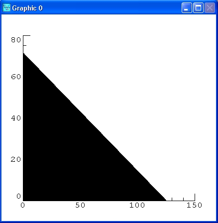
Next we graph the regions specified by the constraints. The last two say that we only need to consider the first quadrant in the x-y plane. Here's a graph delineating the triangular region in the first quadrant determined by the first inequality.
Now let's put in the other two constraint inequalities.
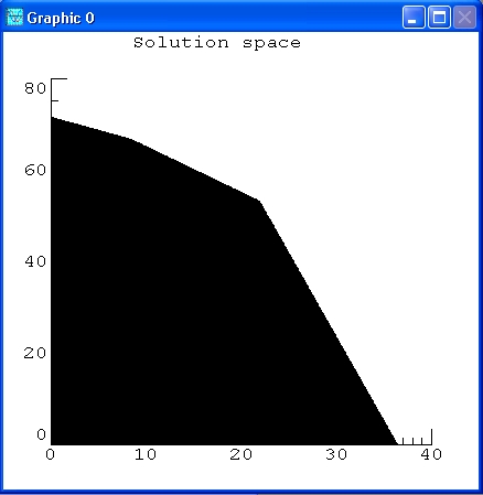
The black area is the solution space that holds valid solutions. This means that any point in this area fulfils the constraints.
Now let's superimpose on top of this picture a contour plot of the objective function P.
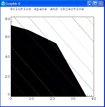
The lines give a picture of the objective function. All solutions that intersect with the black area are valid solutions, meaning that this result also fulfils the set constraints. The more the lines go to the right, the higher the objective value is. The optimal solution or best objective is a line that is still in the black area, but with an as large as possible value.
It seems apparent that the maximum value of P will occur on the level curve (that is, level
line) that passes through the vertex of the polygon that lies near (22,53).
It is the intersection of x + y = 75 and 110*x + 30*y = 4000
This is a corner point of the diagram. This is not a coincidence. The simplex algorithm, which is used
by lp_solve, starts from a theorem that the optimal solution is such a corner point.
In fact we can compute the result:
> x = [1 1; 110 30] \ [75; 4000]
x =
   21.8750
   53.1250
The acreage that results in the maximum profit is 21.875 for wheat and 53.125 for barley. In that case the profit is:
> format bank
> P = [143 60] * x
P =
 6315.63
That is, $6315.63.
Note that these command are in example3.lml
Now, lp_solve comes into the picture to solve this linear programming problem more generally. After that we will use it to solve two more complicated problems involving more variables and constraints.
For this example, we use the higher-level script lp_maker to build the model and then some lp_solve API calls to retrieve the solution. Here is again the usage of lp_maker:
> use sqlpsolve
> help lp_maker

 LP_MAKER  Makes mixed integer linear programming problems.

   SYNOPSIS: lp_handle = lp_maker(f,a,b,e,vlb,vub,xint,scalemode,setminim)
      make the MILP problem
        max v = f'*x
          a*x <> b
            vlb <= x <= vub
            x(int) are integer

   ARGUMENTS: The first four arguments are required:
            f: n vector of coefficients for a linear objective function.
            a: m by n matrix representing linear constraints.
            b: m vector of right sides for the inequality constraints.
            e: m vector that determines the sense of the inequalities:
                      e(i) < 0  ==> Less Than
                      e(i) = 0  ==> Equals
                      e(i) > 0  ==> Greater Than
          vlb: n vector of non-negative lower bounds. If empty or omitted,
               then the lower bounds are set to zero.
          vub: n vector of upper bounds. May be omitted or empty.
         xint: vector of integer variables. May be omitted or empty.
    scalemode: Autoscale flag. Off when 0 or omitted.
     setminim: Set maximum lp when this flag equals 0 or omitted.

   OUTPUT: lp_handle is an integer handle to the lp created.
Now let's formulate this model with lp_solve:
> use sqlpsolve
> f = [143 60];
> A = [120 210; 110 30; 1 1];
> b = [15000; 4000; 75];
> lp = lp_maker(f, A, b, [-1; -1; -1], [], [], [], 1, 0);
> solvestat = sqlpsolve('solve', lp)
solvestat =
    0.00
> format bank
> obj = sqlpsolve('get_objective', lp)
obj =
 6315.63
> format short
> x = sqlpsolve('get_variables', lp)
x =
   21.8750
   53.1250
> sqlpsolve('delete_lp', lp);
Note that these command are in example4.lml
With the higher-level script lp_maker, we provide all data to lp_solve. lp_solve returns a handle (lp) to the created model. Then the API call 'solve' is used to calculate the optimal solution of the model. The value of the objective function is retrieved via the API call 'get_objective' and the values of the variables are retrieved via the API call 'get_variables'. At last, the model is removed from memory via a call to 'delete_lp'. Don't forget this to free all memory allocated by lp_solve.
The solution is the same answer we obtained before.� Note that the non-negativity constraints are accounted implicitly because variables are by default non-negative in lp_solve.
Well, we could have done this problem by hand (as shown in the introduction) because it is very small and it
can be graphically presented.
Now suppose that the farmer is dealing with a third crop, say corn, and that the corresponding data is:
cost per acre $150.75 yield per acre 125 bushels profit per bushel $1.56
With three variables it is already a lot more difficult to show this model graphically. Adding more variables makes it even impossible because we can't imagine anymore how to represent this. We only have a practical understanding of 3 dimentions, but beyound that it is all very theorethical.
If we denote the number of acres allotted to corn by z, then the objective function becomes:
P = (110)(1.30)x + (30)(2.00)y�+ (125)(1.56) = 143x + 60y + 195z
And the constraint inequalities are:
120x + 210y + 150.75z <= 15000
110x + 30y + 125z <= 4000
x + y + z <= 75
x >= 0,�y >= 0, z >= 0
The problem is solved with lp_solve as follows:
> use sqlpsolve
> f = [143 60 195];
> A = [120 210 150.75; 110 30 125; 1 1 1];
> b = [15000; 4000; 75];
> lp = lp_maker(f, A, b, [-1; -1; -1], [], [], [], 1, 0);
> solvestat = sqlpsolve('solve', lp)
solvestat =
     0
> format bank
> obj = sqlpsolve('get_objective', lp)
obj =
 6986.84
> format short
> x = sqlpsolve('get_variables', lp)
x =
    0.0000
   56.5789
   18.4211
> sqlpsolve('delete_lp', lp);
Note that these command are in example5.lml
So the farmer should ditch the wheat and plant 56.5789 acres of barley and 18.4211 acres of corn.
There is no practical limit on the number of variables and constraints that Sysquake can handle. Certainly none that the relatively unsophisticated user will encounter.�Indeed, in many true applications of the technique of linear programming, one needs to deal with many variables and constraints.�The solution of such a problem by hand is not feasible, and software like Sysquake is crucial to success.�For example, in the farming problem with which we have been working, one could have more crops than two or three. Think agribusiness instead of family farmer.�And one could have constraints that arise from other things beside expenses, storage and acreage limitations. For example:
Below is a sequence of commands that solves exactly such a problem. You should be able to recognize the objective expression and the constraints from the data that is entered.� But as an aid, you might answer the following questions:
> use sqlpsolve
> f = [110*1.3 30*2.0 125*1.56 75*1.8 95*.95 100*2.25 50*1.35];
> A = [120 210 150.75 115 186 140 85;
        110 30 125 75 95 100 50;
        1 1 1 1 1 1 1;
        1 -1 0 0 0 0 0;
        0 0 1 0 -2 0 0;
        0 0 0 -1 0 -1 1];

> b = [55000;40000;400;0;0;0];
> lp = lp_maker(f, A, b, [-1; -1; -1; -1; -1; -1], [10 10 10 10 20 20 20], [100 Inf 50 Inf Inf 250 Inf], [], 1, 0);
> solvestat = sqlpsolve('solve', lp)
solvestat =
     0
> format bank
> obj = sqlpsolve('get_objective', lp)
obj =
 75398.04
> format short
> x = sqlpsolve('get_variables', lp)
x =
   10.0000
   10.0000
   40.0000
   45.6522
   20.0000
  250.0000
   20.0000
> sqlpsolve('delete_lp', lp);
Note that these command are in example6.lml
Note that we have used in this formulation the vlb and vub arguments of lp_maker. This to set lower and upper bounds on variables. This could have been done via extra constraints, but it is more performant to set bounds on variables. Also note that Inf is used for variables that have no upper limit. This stands for Infinity.
Note that despite the complexity of the problem, lp_solve solves it almost instantaneously. It seems the farmer should bet the farm on crop number 6.�We strongly suggest you alter the expense and/or the storage limit in the problem and see what effect that has on the answer.
Suppose we want to solve the following linear program using Sysquake:
max 4x1 + 2x2 + x3
s. t. 2x1 + x2 <= 1
x1 + 2x3 <= 2
x1 + x2 + x3 = 1
x1 >= 0
x1 <= 1
x2 >= 0
x2 <= 1
x3 >= 0
x3 <= 2
Convert the LP into Sysquake format we get:
f = [4 2 1]
A = [2 1 0; 1 0 2; 1 1 1]
b = [1; 2; 1]
Note that constraints on single variables are not put in the constraint matrix. lp_solve can set bounds on individual variables and this is more performant than creating additional constraints. These bounds are:
l = [ 0 0 0]
u = [ 1 1 2]
Now lets enter this in Sysquake:
> use sqlpsolve
> f = [4 2 1];
> A = [2 1 0; 1 0 2; 1 1 1];
> b = [1; 2; 1];
> l = [ 0 0 0];
> u = [ 1 1 2];
Now solve the linear program using Sysquake: Type the commands
> lp = lp_maker(f, A, b, [-1; -1; -1], l, u, [], 1, 0);
> solvestat = sqlpsolve('solve', lp)
solvestat =
     0
> obj = sqlpsolve('get_objective', lp)
obj =
    2.5000
> x = sqlpsolve('get_variables', lp)
x =
    0.5000
    0.0000
    0.5000
> sqlpsolve('delete_lp', lp);
What to do when some of the variables are missing ?
For example, suppose there are no lower bounds on the variables. In this case define l to be the empty set using the Sysquake command:
> l = [];
This has the same effect as before, because lp_solve has as default lower bound for variables 0.
But what if you want that variables may also become negative?
Then you can use -Inf as lower bounds:
> l = [-Inf -Inf -Inf];
Solve this and you get a different result:
> use sqlpsolve
> lp = lp_maker(f, A, b, [-1; -1; -1], l, u, [], 1, 0);
> solvestat = sqlpsolve('solve', lp)
solvestat =
     0
> obj = sqlpsolve('get_objective', lp)
obj =
    2.6667
> x = sqlpsolve('get_variables', lp)
x =
    0.6667
   -0.3333
    0.6667
> sqlpsolve('delete_lp', lp);
Note that everwhere where lp is used as argument that this can be a handle (lp_handle) or the models name.
These routines are not part of the lpsolve API, but are added for backwards compatibility. Most of them exist in the lpsolve API with another name.
Under Windows, the sqlpsolve Sysquake driver is a dll: sqlpsolvext.dll
Under Unix/Linux, the sqlpsolve Sysquake driver is a shared library.: sqlpsolvext.so
This driver is an interface to the lpsolve library lpsolve55.dll/liblpsolve55.so that contains the implementation of lp_solve.
lpsolve55.dll/liblpsolve55.so is distributed with the lp_solve package (archive lp_solve_5.5.2.5_dev.zip/lp_solve_5.5.2.5_dev.tar.gz).
The sqlpsolve Sysquake driver is just a wrapper between Sysquake and lp_solve to translate the input/output to/from Sysquake and the lp_solve library.
The sqlpsolve Sysquake driver is written in C. To compile this code, under Windows the Microsoft visual C compiler is needed and under Unix/Linux the standard cc compiler.
The needed commands are in a batch file/script.
Under Windows it is called cvc.bat, under Unix/Linux ccc.
In a command prompt/shell, go to the lpsolve Sysquake directory and enter cvc.bat/sh ccc
and the compilation is done. The result is sqlpsolvext.dll/sqlpsolvext.so.
See also Using lpsolve from MATLAB, Using lpsolve from O-Matrix, Using lpsolve from Scilab, Using lpsolve from Octave, Using lpsolve from FreeMat, Using lpsolve from Euler, Using lpsolve from Python, Using lpsolve from Sage, Using lpsolve from PHP, Using lpsolve from R, Using lpsolve from Microsoft Solver Foundation