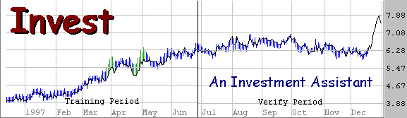
Invest - An Investment Assistant
6.038 Final Project - AI in Practice
Manolis Kamvysselis - Shishir Mehrotra - Nimrod Warshawsky
manoli@mit.edu - shishir@mit.edu - nimrodw@mit.edu
This paper describes our attempt at implementing a stock price prediction system implementing various AI techniques. We found relatively poor performance across the gamut of techniques attempted. We conclude that stock prices are a random walk across the general mean of the system. Therefore, we propose that it is virtually impossible to predict with a high degree of certainty how a stock price will perform in the future.
The of the project is to build an investment assistant. The purpose is not to have the computer secretely predict the output of a stock, but to use the computational power of computers and the methods learned in Artificial Intelligence in practice, in the domain of the stock market. The system is to help an investor make predictions on the future of a stock, based on the history of the market.
There are many ways of approaching this problem. Programs have been written to manage entire portfolios. In our case, the user chooses a set of stocks to predict, and a set of stock histories to predict these stocks from. The system is then to make predictions using different AI methods, and judge its competence based on the actual data from the stock market.
More precisely, a program can predict either the future of a single stock, or of a set of stocks. Also, it can predict either an absolute stock price, or the sign of the derivative, that is if the stock will go up or down. Finally, the program can either predict the short-run outputs, or the long-range behavior of the stock.
Each of these alternatives corresponds to a different type of investment strategies. The user might be interested in investing in many stocks if they go up over a long period of time, or he/she may be interested in a few quick investments of stocks that are going to go really high in a short time.
There are different ways of approaching the problem, and they reflect different theories of how the market works. The assumption of the project is that there is a certain correlation between past stock prices and future behavior of the market.
Of course, other factors affect the stock market, such as political decisions, economical trends, hurricanes, international trade, boycotts and strikes. Since we don't have that data, we can either assume that it is reflected in the history of the market (for example that it is the low prices of a companie's stocks that caused a strike, or that the economic trends which caused the strike are reflected in the stock market history). Alternatively, we can affirm from the start that our program will not predict accurately such changes in the stock market.
Two different predictors were built on these assumptions. The first one is a Neural Net predictor, that can handle highly non-linear relations between history and future of the stock market. The second one is a Nearest Neighbor predictor, which assumes that linearly similar histories should yield similar results. Finally, a third kind of predictor was designed and implemented, but never tested, trying to pay attention to only those points of the market which seemed important
What we expect to gain out of the project is not a program that is going to make billions (thus avoiding the case of a program that is going to waste billions). First of all, we're not building a program that will be left alone playing on the stock market. Instead we're building an assistant that will advise Investors on what the correlations are between stocks, and that can throw computational power directed by a human's insights.
We understand that if predicting the market was such a simple task that a simple neural net could predict it, then people wouldn't be trying to make money on it anymore, since everybody would just know the solution. Moreover, in an environment like the stock market, when everyone has found the solution and is making money on the stock market, the solution irremediably changes, becoming how to beat the others who are using that particular solution. It is therefore both in practice and in theory an intractable problem.
Then why attack a problem for which we know there is no solution as a final project for a class? First, because of our interest in the stock market business, and to gain some hands-on experience in building a stock market predictor. More importantly though, we are here to learn, and doing this project we learned a great deal about AI in practice.
In designing the new Neural Network code, it was important to ensure efficiency for feeding the network forward, as well as a relatively efficient way of handling the data structure's elements. The design choice involved building ontop of certain of the BPNN neural net code provided by CMU, while completely rewriting and building on top of other parts.
The decision to use the BPNN code stemmed from the fact that it was a relatively robust system with free access to the source code. Furthermore, it had some functionality that was elegantly implemented. BPNN has an incredibly simple way of handling saved nets. However, its handling of weights and feed forwarding were incredibly inefficient. The first optimization involved modifying their squash from being a function, to being an inline define. The second modification involved rewriting their feed forward code. Feed forward is a function that is called an awesome number of times during neural net use. Therefore, the number of function calls that feed forward places are minimized. This leads to tighter code that is quite readable.
Training the net was yet another issue. We knew that the size of these nets could become excessively large, and were concerned that training of the nets using standard backprop would be painfully slow. Therefore a conjugate gradient method was implemented.
Conjugate gradient is a minimizing function that relies on the value of a function as well as the value of its gradient. The value of the gradient is calculated as described in Nimrod's individual paper. However conjugate gradient relies on calculation of error over all of the training samples. This required a fundamental change in how the BPNN neural net data structure was handled. Because backprop can be trained incrementally as training samples are introduced there is no need to store the entire sample set. However, conjugate gradient does require storing the entire set and changes how samples must be handled. The current implementation stores the entire input set in RAM, thereby allowing for very quick training. The choice of storing the input set in RAM restricts how large the training set is allowed to grow. Though it was feared this would be a lethal constraint, we found that the available resources were more than sufficient to handle the set we were using.
The use of the Numerical Recipes for C code to handle the conjugate gradient algorithm proved to be an excellent choice. Though there was a decent amount of work in designing an interface between the expanded neural net code and the format that the numerical recipes code expected, the transition was relatively seamless requiring only the changing of the types used in the function data structures.
Inputs to the neural net are open-ended depending on what factors are chosen and how the space is used. The only requirement is that the input values be between 0 and 1. This proved to be a very tricky problem, however, since our scaling caused some numbers to appear inconsequential. We suspect this is one of the major causes of poor convergence in some of the nets. For example some nets show a phenomenally small output error, however when one examines the output, it becomes apparent that the net and the target output are poorly correlated. However, upon further inspection, many of these poor convergences can be explained by examining the values of the output nodes. Since the error is the sum of the squares of the output nodes, a difference of 10e-3 actually becomes a difference of 10e-6. It would appear that a difference of 10e-3 is inconsequential, but when the price of the feature varies from 4*10e-2 to 5*10e-2, it becomes apparent that this "inconsequential" difference is in fact very large. We recognized some methods of dealing with this problem, however, chose to avoid them for simplicity. Some solutions include changing the nodes in the net to linear functions instead of the sigmoid, or scaling different factors differently.
The arrangement of inputs to the neural net was relatively consistent. To describe the system I will present a simplified net. Assume that we are concerned in predicting IBM's stock tomorrow based on IBM's value today and yesterday, as well as Dell's stock today and yesterday. In our encoding system this leads to 2 factors (IBM and Dell) with each factor having a "history" of 2 (today and yesterday). Therefore, the input of the neural net includes 4 nodes. The output of the neural net is simply IBM's value tomorrow which is encoded in a single output node.
Changing of the net size did not have a magnificent effect on output. We settled on a neural net that had a hidden level of 16 hidden nodes.
The reason to try Nearest Neighbors is that there is no need for training. The concept is simple: For every output, the prediction of the next value is simply the output of that feature vector whose input is the closest to the input values. In that case, closest means that the sum of differences between the two feature vectors is minimal.
The advantage of a Nearest Neighbor approach to prediction is that the user can change portfolios and immediately get a predictive result, without wasting time in training. If the result seems promising, then a neural net (or other predictive measure) can be used to verify the "goodness" of a new portfolio.
Characteristics of the Stock Market
The pattern matching alternative to Neural Nets and Nearest Neighbors was built based on the following assumptions on the Stock Market Characteristics:Features and Design Criteria in the Pattern Matching code
To address those problems, the current design is as follows: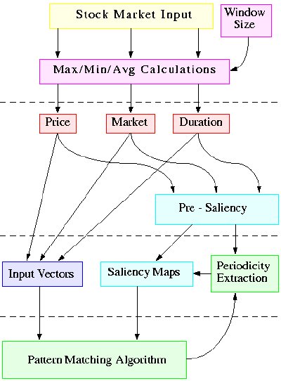 |
Input Layer The input provided by the stock quotes is preprocessed to calculate a Price value, a Market index, and a Duration elapsed between the time of the input and the current time. Maximum, minimum, and average values within a window are calculated for each of them, to normalize the data passed on to the next layer. Saliency Layer Based on these values and their maximums, minimums and averages, saliency values are calculated for each piece of data and their derivatives. This results in saliency maps which make certain vectors stand out, based on how important they are in predicting the stock market. Pattern Matching The pattern matching algorithm will be biased in matching the values which are salient on the vectors which are salient. Patterns of varying lengths will be stored for salient vectors, and matched as new inputs come in. Prediction When a pattern is matched partially with the current input, the system will predict future input as the continuation of the stored pattern. Since more than one patterns will be matched (at least one for each pattern length), a weighted average will be calculated, depending on certainty and pattern length. |
Market Value and Duration Elapsed
The market and duration fields supplement the stock value, by providing information otherwise not contained in the succession of values. The market index represents the state of the market at the time the stock was quoted.
The duration elapsed is the time difference between the current time and the time of the stock. When a pattern of 5 consecutive stocks is constructed, the duration fields will be [4, 3, 2, 1, 0], and they will match exactly any other pattern of consecutive stocks. However, there is no constraint on which data will enter a pattern.
For example, a pattern table can have the first element come from stock X, the second from stock Y, and the third from stock Z. A pattern in that table could be "stock X falls 2 days ago, stock Y rises 10 days ago, and stock Z has maximum value now". In that case the duration fields will be [2, 10, 1] for stocks [x y z]. The pattern will also match [2, 8, 1], where Y rose 8 days ago instead. This allows the system to match a larger class of patterns independent of the exact time of occurence, and what type of stocks are involved.
If such a duration field is not included, one has to train the system to recognize only cases where a stock depends on exact time relationships. This varying duration field allows for more dynamic relationships between stocks. Since pattern tables are created dynamically, depending on what data is salient, the relationships to look for need not be hard-coded. A different pattern table will be created for different combinations of stocks, but that's another story, which belongs to the pattern matching domain.
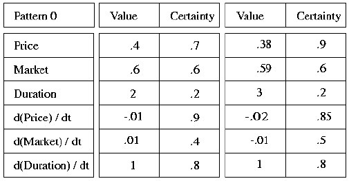
Augmented Input Vector
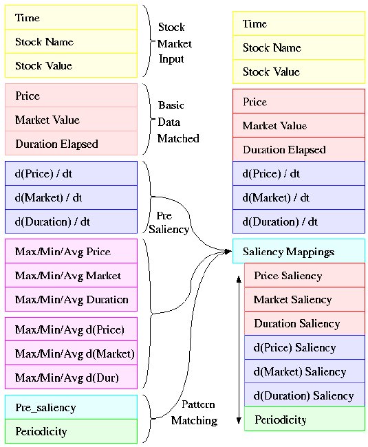
On the diagram to the left, the yellow boxes represent the data received by an individual stock quote. In the red boxes lies the transformed data, as described above, that will be used in matching patterns. The stock value becomes the price (after some normalization). The time is encoded in the duration elapsed. A general value of the stock market at the time of the stock quote is encoded in the Market Value. The stock name is not matched within the pattern element, but is encoded in the pattern table. Within a pattern table, the same element will always come from the same stock X.
The input vector is augmented by the derivatives of the three basic values, represented in blue. Only the basic values and their derivatives are matched when comparing elements. The saliency values are simply there to determine what is important when making a match, but they are not matched themselves.
Temporarily, maximum, minimum and average values of each of the six fields are calculated for the window-size (magenta), and they are used to calculate the saliency maps (cyan). The window size represents how far back in the past we should look for normalizing values when comparatively analyzing the current data. It is relative to those min max and avg values that values are matched within patterns, as will be described later on. They also serve as a normalization step, so that data given in different units can be compared in an unbiased way.
Along with the other saliencies, a periodicity saliency is calculated, which makes salient vectors based on a periodically salient history (green).
Thus we have reached from a 3-value input (time, name, value) a 6-value vector (value, market, duration and derivatives) to match upon. Each vector also has a 7-field saliency, which determines what values should be matched more carefully.
Vector Saliency
Saliency is a value between 0 and 1 that indicates how important a field inside a vector is. The most important ones have a value of 1, the least important, a saliency of 0.
The saliency value for a vector is computed as the average of individual saliencies calculated for each of the components. A vector saliency is also between 0 and 1.
Individual Saliencies
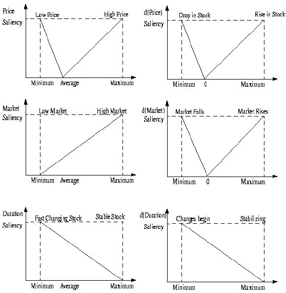
Individual saliencies for each value are computed relative to the window of attention. The highest value in the window will generally have a saliency value of 1, as well as the lowest one. An average value will have a saliency value of 0. The distribution was made linear in between for reasons of simplicity.
For example, one should pay attention to a stock when it's at its maximum value. Similarly important are the moments when the stock is at its minimum value. However, when the stock is just an average value, no special attention should be paid to that particular point in time.
Similarly, a maximally rising stock will be salient (highest stock value derivative), just as a maximally falling stock. A stable stock will have a derivative of 0, and a saliency of 0 accordingly.
The market saliency functions in the same way more or less, only the system is now biased to paying attention to high-markets. The duration saliency is biased to those stocks that change faster, as well as those which start changing faster.
These biases can be changed for best performance as the system gets tested. In doing so, insights might be gained about real market behaviors and relationships. The first-order function that is now used in saliencies could also be changed to second order, or gaussian as the system becomes more mature.
Periodicity Saliency
Based on the average of these saliencies, each stock gets a pre-saliency value, which is used to compute the periodicity of the input. This can lead the computer to expect salient stocks at specific times if it has been seeing them periodically. Hence, if falling on a periodically salient time, even a non-salient stock could appear important and be recorded in a pattern.
Pattern matching, along with learning the periodicity of the input, does the basic computations the code is based upon. It is able to learn patterns of different length from the input, and match partially completed patterns to either predict future inputs, or turn the focus of attention to different patterns interesting to a specific behavior.
The pattern matcher receives commands from the attention loop, which directs it on what to match, what to record (learn), and what to pay attention to.
Saliency Maps
We have thus constructed many saliency maps which can make different vectors stand out, depending on what feature one is paying attention to. One can pay attention to stocks salient in price, or its derivative, or in a high market envirnoment, or a rapidly changing market, or a rapidly changing stock, or a stock which starts changing. The pattern matcher also computes a periodicity saliency map, which gives a value of 1 to stocks expected to be salient, and a 0 to the non-salient ones. Together with the pre-saliency values, this final addition completes the saliency maps constructed on the input.
Pattern Tables
The figure shows an individual pattern of two elements. A pattern table will hold many such patterns. A different pattern table is created for every pattern length that we are matching. Moreover, for the same length (the same number of elements that we match upon), there will be different pattern tables for different stock combinations. For patterns of 3 elements for example, we can have a pattern table storing all patterns found on [x y z] another one storing all patterns found on [a b z], and so on.Pattern Matching
Pattern matching, along with learning the periodicity of the input, does the basic computations the code is based upon. It is able to learn patterns of different length from the input, accross different stocks. A match partially completed can predict future inputs, or turn the focus of attention to different patterns interesting to specific markets behavior.
Calculating Certainties
Every time a pattern is matched, individual elements get averaged, (weighted by the number of inputs each value has matched), and their certainties are updated. The certainty of a match between two values is one minus the ratio of differences between the two values and the maximum and minimum values at the current window. The certainty of a match between two pattern elements is the average of the certainties of their values. The certainty of a match between two patterns, is the average of the certainties of their elements, weighted by the saliency of each element. Intuitively, one will try to match within a sequence of stock the important features, and will care less about less salient features which do not match.
Updating Values
When the certainty with which two patterns are matched is too low, then a new pattern is added to the pattern table. When the certainty is high enough, then the matched pattern is extended to include the current pattern with which it matched.
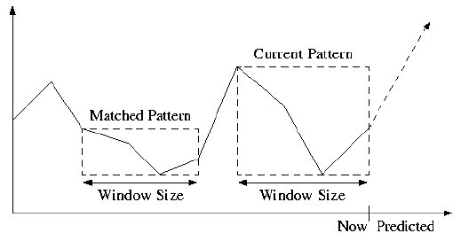
Normalizing for a Match
Let's consider a simple example where all elements of a pattern are consecutive stock values of the same stock.
In the figure, we would like that the second pattern enclosed in the box matches the first one, previously recorded. Clearly, the values do not match, nor do their derivatives, since everything seems to have doubled (for example in volume).
Therefore, when a match is made, what is compared is not absolute values, but instead values relative to the current maximum and minimum of the window-size considered.
Making a Prediction
Predictions are made accordingly, relative to the current window maximum and minimum. If the current pattern has length 4, then the system will match the first 4 elements of a stored pattern of length 5, and predict the next stock as the final element of the matched stored pattern.
Patterns of different sizes are matched in making the predictions. Their predictions are weighted then averaged, to obtain the final prediction. For each length, let best[length] be the pattern of that length that best matched the current pattern (of length-1). Each best[length] will have a certainty value associated with it, and with each element. This certainty value, along with the pattern length, are used in weighting the different size predictions.
The longer the length of the pattern is, the higher its weight should be. The reason for this bias of trusting longer patterns is that they are less likely to match. For almost anything, a two-stock pattern will match with high certainty.
The system was never tested on actual stock market input. It was tested on hand-written patterns, and it successfully recognized them and matched them. If such patterns exist in the stock market was thus something we were not able to assert.
A major concern i have for the system's success is about the progressively decreasing certainty values for each of the patterns as more and more vectors are matched. The solution that was envisioned but not implemented was a reordering of the pattern table after the certainties reach low values. That would take the extreme vectors out of the set of vectors matched with the particular pattern and match the other vectors in the set with one or the other. This would hopefully split the mass of uncertain vectors by splitting its centroid to create smaller and denser sets.
Another problem is that of patterns which start out exactly the same but turn out different. The system will be 100% sure of one prediction when it has matched exactly previous state, and it will be 100% wrong. Solutions to this were tested by increasing the pattern length and decreasing the minimum saliency for considering more inputs, in which a divergence should be found, but such a divergence was not evident. This depended, of course to the specifics of the input fed into the system.
The interface between the middle engine and the neural network code and nearest neighbor code interacted through files. This allowed development to occur concurrently and led to code that was isolated.
Files had a structure as follows: A file includes a header that describes how many features, how many outputs, how long in history the "window" should be opened and how many days total exist in the database. The file is then separated into an "input" set and an "output" set. The rows in the input set correspond to the different features being examined. The columns correspond to different days. The file is read into memory building a table of features against dates. Again, accesses are quite efficient, but introduces some limit onto the input size.
The second step was to represent this data in useful ways. One of our original predictions was that modeling stock prices may be difficult but capturing other secondary information may be easier. Thus the concept of a transofrm was added to the system. These transforms took one set of data and manipulated it to produce a piece of data structured the same way. Some examples of transforms that were used are: shift data, minimum value, maximum value, running averages, etc. These transforms also provided an easy mechanism for producing testing data from training data, it just needed to be shifted over in time.
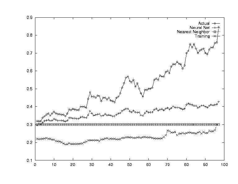
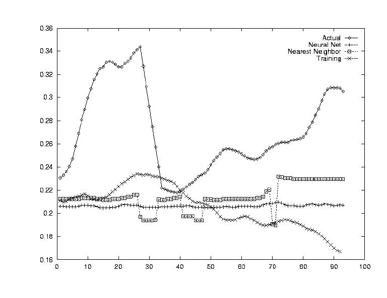
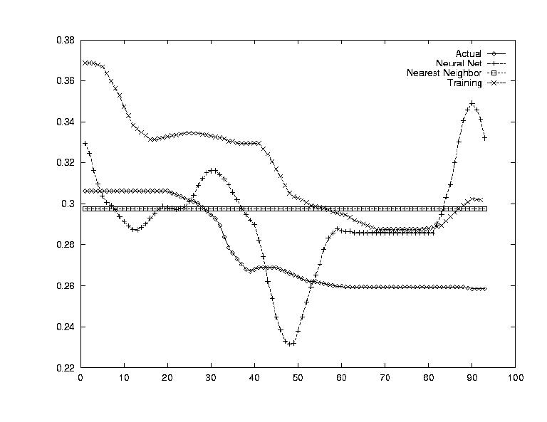
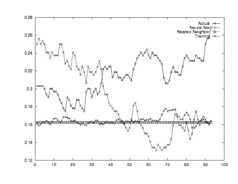
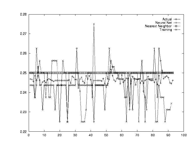
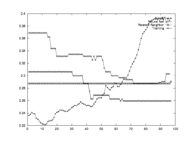
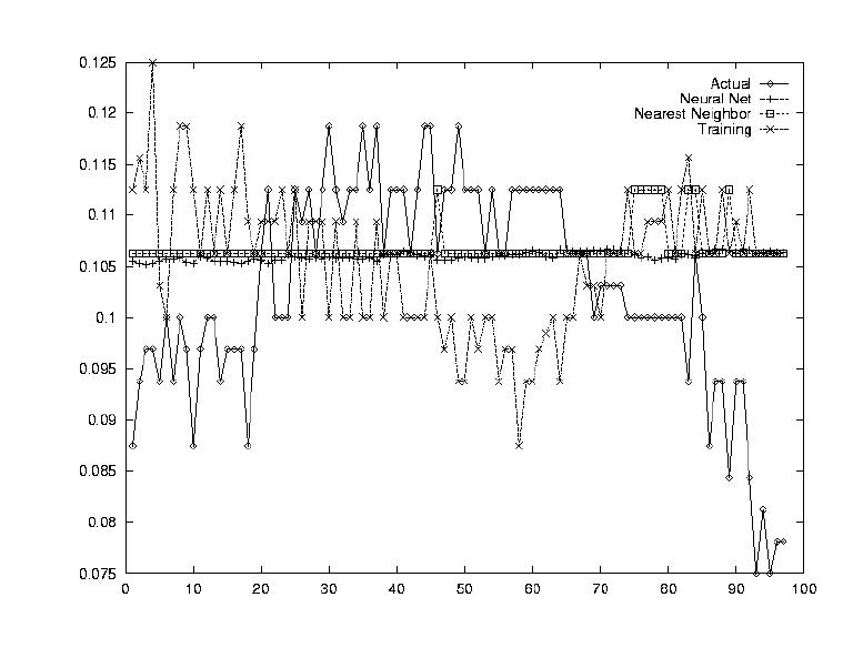
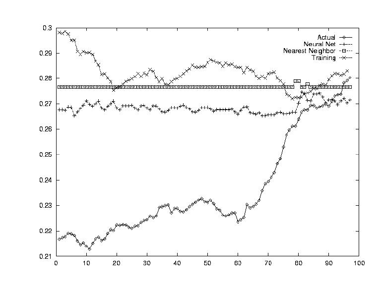
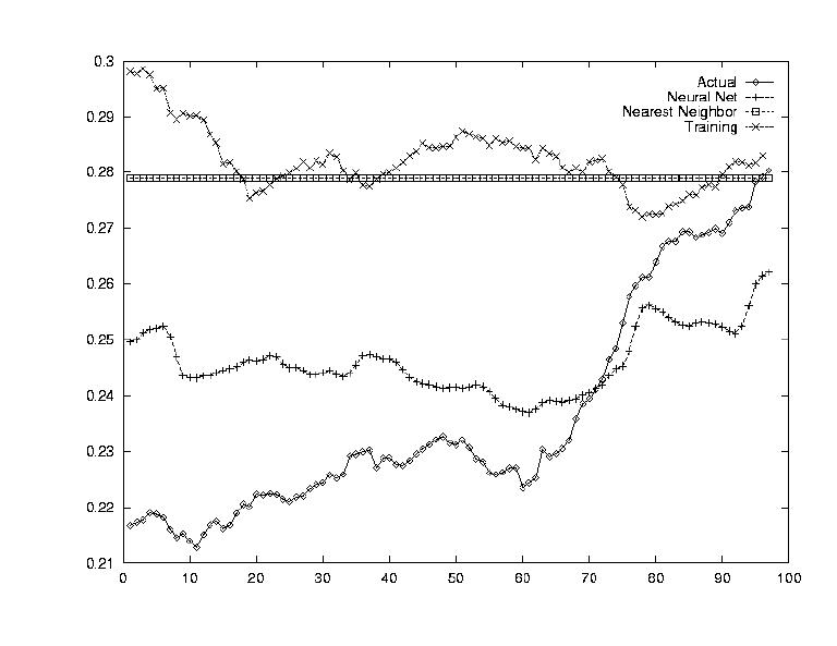
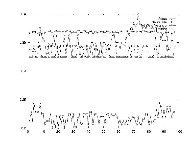
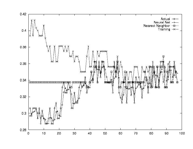
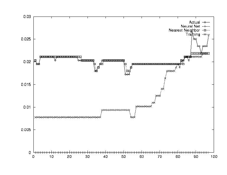
At this point, all of our questions could be answered. The results are summarized below, and for each strategy, three outputs are provided, first one where the system performed poorly, a second one with medium performance, and a third one where the system performed well.
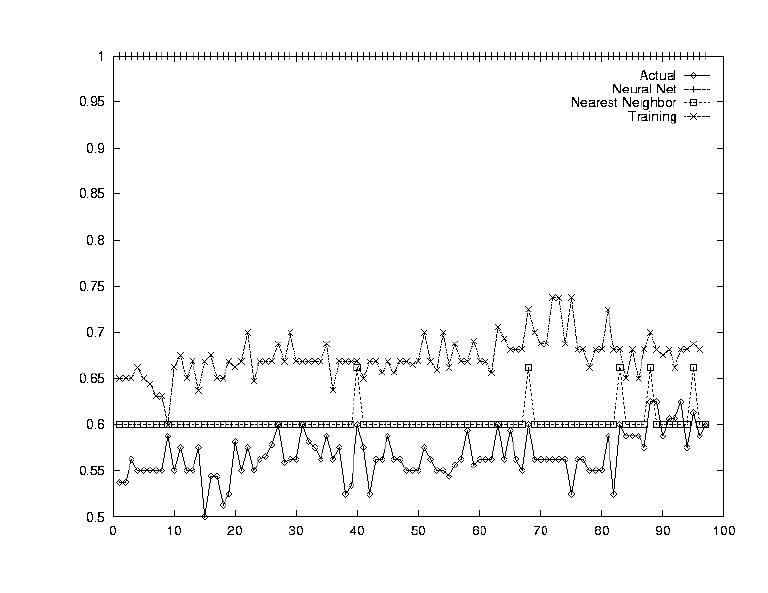
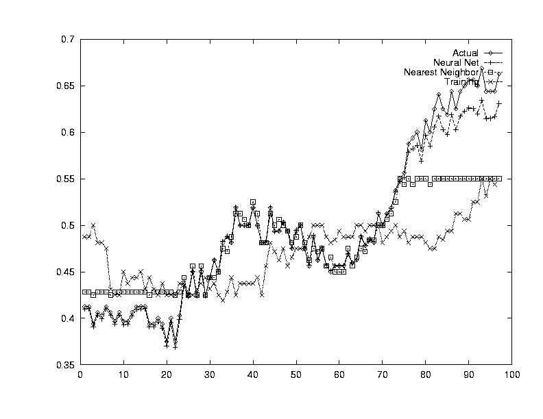
The purpose is to ensure that our system was working in the way we expected. To do this, the inputs to the system were the same as the outputs. All the system had to learn was the identity function.
The neural net performed extremely well. This showed that the Neural Net was definitely capable of modeling such a complex system given enough information.
Nearest Neighbors worked very well but it was expected too. Every piece of training data was the same as the testing data, so it had seen each of the vectors already. It just had to look them up. Again, this test showed us that Nearest Neighbor could work, given a large database of old values.
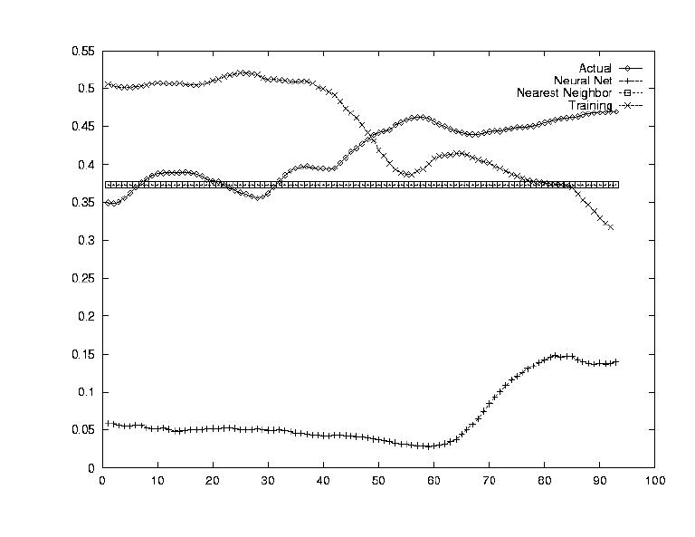
One of the largets problems in predicting stockmarket information is that the data is so erratic. Since the data was sampled on a daily level, this was seen as a huge problem. Thus the stock's value was smoothed out by establishing a running average transform, i.e. computing the average of the next week's data as today's value.

Perhaps one of the most used estimates for a stock's performance is its past performance. Many analysts will say things like, "Last time it went up like this, it came down even harder." Modelling this effect was the subject of this test. A very simple shifting transform was used where day 1's data was replaced by day x's data as day 2's data was replaced by day x+1.
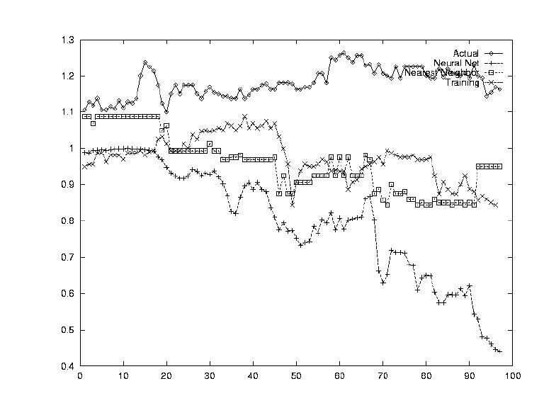
Another indicator of a stock's value which is often used, is the performance of other stocks. The idea is that the stocks act together as a market, and incorporating a market index could be very beneficial. To this end, a sum transform was sued which averaged all the data for the 148 stocks.

The opposite question from Test 4 was asked in this test: how does this one stock determine the market index's value? By testing each stock's correlation against the average computed in Test 4, this correlation could be established.
Having the system output predictions for stock prices is very interesting, but in order to use the information one must know have a strategy. In other words, one could look at the system's predictions and determine when to buy and when to sell. Perhaps a very useful implementation of the system would be to have the system itself report profitable buy days and profitable sell days.
The idea of having strategy be an output can be very complicated. Different types of strategies exist, from ones that capitalize on short term fluctuations to ones that lay in wait of long term trends. For the purpose of demonstrating the possibility of having a strategy output, a very simple strategy model was chosen. Basically, the model said that given a set of predictions, one would pick one day to buy and one day to sell. One would prefer to buy on the lowest price day and to sell on the highest. Thus, as two additional binary outputs (1 - buy/sell, 0 -no buy/ no sell), a simple strategy output was attempted.
(It sure sounds better than failures.)
We were able to predict the stock market (NOT!). Just like we were expecting, the program will not make billions on the stock market. Most of the time it gives a wrong prediction, and sometimes it's really off.
The pattern matching code was never integrated to the system. It worked on hand-written input, but was never tested on actual stock prices.
Our user interface fell in the water as we lost a member of our team.
Our first success was getting 10 years worth of data, in a world where everyone is selling stock quotes at their own price, and trying to keep everyone else from getting to the stock market history.
Another success was getting the neural net and nearest neighbor code integrated with the data, and learning the actual market values. The system was able to predict what it was trained on, and thus effectively exhibited learning.
Finally, we learned a great deal about how team projects should be done, and the mistakes ones should avoid. We learned about training Neural Nets and the conjugate gradient method of training. We learned about nearest neighbors and its limitations.
The most important lesson we come out of this project with however, is that the stock market is not an easy thing to predict, and that simple AI algorithms cannot effectively extract the important information out of it. Either more complicated algorithms should be devised to predict the stock market, or more data should be accounted for in the prediction.
The short term behavior of the market seems to be more or less random, and one should be interested more in larger patterns, possibly by smoothing out the data to eliminate high-frequency noise.
A simple advise to those betting money on stock market computer systems would simply be "Don't!"
Now that the system is built and manages real data, different engines can be incorporated and tested. Different algorithms might have greater prediction power, perhaps in predicting other types of values (integrals, derivatives, combinations of prices), or based on other types of values (hurricane rate, political movements).