CHAPTER 1:  GENOME CORRESPONDENCE

1.1. Introduction

The first issue in comparative genomics is determining the correct correspondence of chromosomal segments and functional elements across the species compared.  This involves the recognition of orthologous segments of DNA that descend from the same region in the common ancestor of the species compared.  However, it is equally important to recognize which segments have undergone duplication events, and which segments were lost since the divergence of the species.  By accounting for duplication and loss events, we ensure that we are comparing orthologous segments.

We decided to use genes as discrete genomic anchors in order to align and compare the species.  We constructed a bipartite graph connecting annotated protein-coding genes in S. cerevisiae to predicted protein-coding genes in each of the other species based on sequence similarity at the amino-acid level.  This bipartite graph should contain the orthologous matches but also contains spurious matches due to shared domains between proteins of similar functions, and gene duplication events that precede the divergence of the species.  Determining which matches represent true orthologs and resolving the correspondence of genes across the four species will be the topic of this chapter.

We present an algorithm for comparative annotation that has a number of attractive features.  It uses a simple and intuitive graph theoretic framework that makes it easy to incorporate additional heuristics or knowledge about the genes at hand.  It represents matches between sets of genes instead of only one-to-one matches, thus dealing with duplication and loss events in a very straightforward way.  It uses the chromosomal positions of the compared genes to detect stretches of conserved gene order and uses these to resolve additional orthologous matches.  It accounts for all genes compared, resolving unambiguous matches instead of simply best matches, thus ensuring that all 1-to-1 genes are true orthologs.  It works at a wide range of evolutionary distances, and can cope with unfinished genomes containing gaps even within genes. 

1.2. Establishing gene correspondence

Previously described algorithms for comparing gene sets have been widely used for various purposes, but they are not applicable to the problem at hand. 

Best Bidirectional Hits (BBH)^30,31 looks for gene pairs that are best matches of each other and marks them as orthologs.  In the case of a recent gene duplication however, only one of the duplicated genes will be marked as the ortholog without signaling the presence of additional homologs.  Thus, no guarantees are given that 1-to-1 matches will represent orthologous relations and incorrect matches may be established.

Clusters of Orthologous Genes (COG)^32,33 goes a step further and matches groups of genes to groups of genes.  Unfortunately, the grouping is too coarse, and clusters of orthologous genes typically correspond to gene families that may have expanded before the divergence of the species compared.  This inability to distinguish recent duplication events from more ancient duplication events makes it inapplicable in this case, since the genome of S. cerevisiae contains hundreds of gene pairs that were anciently duplicated before the divergence of the species at hand³⁴.  COGs would not distinguish between the two copies of anciently duplicated genes, and many orthologous matches would not be detected (Koonin, personal communication).

We introduce the concept of a Best Unambiguous Subset (BUS), namely a group of genes such that all best matches of any gene within the set are contained within the set, and no best match of a gene outside the set is contained within the set.  A BUS builds on both BBHs and COGs to resolve the correspondence of genes across the species.  The algorithm, at its core, represents the best match of every gene as a set of genes instead of a single best hit, which makes it more robust to slight differences in sequence similarity.  A BUS can be isolated from the remainder of the bipartite gene correspondence graph while preserving all potentially orthologous matches.  BUS also allows a recursive application grouping the genes into progressively smaller subsets and retaining ambiguities until later in the pipeline when more information becomes available.  Such information includes the conserved gene order (synteny) between consecutive orthologous genes that allows the resolving of additional neighboring genes.

1.3. Overview of the algorithm

We formulated the problem of genome-wide gene correspondence in a graph-theoretic framework.  We represented the similarities between the genes as a bipartite graph connecting genes between two species.  We weighted every edge connecting two genes by the amino acid sequence similarity between the two genes, and the overall length of the match. 

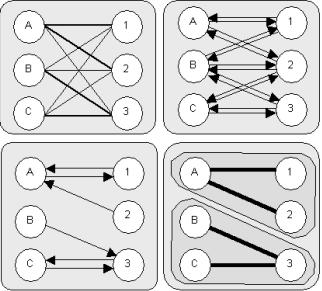We separated this graph into progressively smaller subgraphs until the only remaining matches connected true orthologs (Figure 1.1).  To achieve this separation, we eliminated edges that are sub-optimal in a series of steps.  As a pre-processing step, we eliminated all edges that are less than 80% of the maximum-weight edge both in amino acid identity and in length.  Based on the unambiguous matches that resulted from this step, we built blocks of conserved gene order (synteny) when neighboring genes in one species had one-to-one matches to neighboring genes in the other species; we used these blocks of conserved synteny to resolve additional ambiguities by preferentially keeping matches within synteny blocks.  We finally searched for subsets of genes that are locally optimal, such that all best matches of genes within the group are contained within the group, and no genes outside the group have matches within the group.  These best unambiguous subsets (BUS) ensure that the bipartite graph is maximally separable, while maintaining all possibly orthologous relationships.

When no further separation was possible, we returned the connected components of the final graph.  These contain the one-to-one orthologous pairs resolved as well as sets of genes whose correspondence remained ambiguous in a small number of homology groups.

1.4. Automatic annotation and graph construction

In this section, we describe the construction of the weighted bipartite graph G, representing the gene correspondence across the species compared.  We started with the genomic sequence of the species and the annotation of S. cerevisiae, namely the start and stop coordinates of genes.  We then predicted protein-coding genes for each newly sequenced genome.  Finally we connected across each pair of species the genes that shared amino-acid sequence similarity.

The input to the algorithm is based on the complete genome for each species compared.  For S. cerevisiae, we used the public sequence available from the Saccharomyces Genome Database (SGD) at genome-www.stanford.edu/Saccharomyces.  SGD posts sixteen uninterrupted sequences, one for each chromosome.  The sequence was obtained by an international sequencing consortium and published in 1996.  It was completed by a clone-based sequencing approach and directed sequence finishing to close all gaps.  Subsequent to the publication, updates to the original sequence have been incorporated in SGD based on resequencing of regions studied in labs around the world.

The genome sequence of S. paradoxus, S. mikatae and S. bayanus was obtained at the MIT/Whitehead Institute Center for Genome Research.  We used a whole-genome shotgun sequencing approach with paired-end sequence reads of 4kb plasmid clones, with lab protocols as described at www-genome.wi.mit.edu.  We used ~7-fold redundant coverage, namely every nucleotide in the genome was contained on average in at least 7 different reads.  The information was then assembled with the Arachne computer program^35,36 into a draft sequence for each genome.  The assembly contains contigs, namely continuous blocks of uninterrupted sequence, and scaffolds or supercontigs, namely uninterrupted blocks of linked contigs for which the relative order and orientation is known.  This order and orientation is given by the pairing of reads that originated from the ends of the same 4kb clone.  The draft genome sequence of each species has long-range continuity (more than half of the nucleotides are in scaffolds of length 230-500 kb, as compared to 942 kb for the finished sequence of S. cerevisiae), relatively short sequence gaps (0.6-0.8 kb, which is small compared to a typical gene), and contains the vast majority of the genome (~95%). 

Once the genome sequences are available, we determine the set of protein-coding genes for each species.  For S. cerevisiae, we used the public gene catalogue at SGD.  It was constructed by including all predicted protein coding genes of at least 100 AA that do not overlap longer genes by more than 50% of their length.  It was subsequently updated to include additional short genes supported by experimental evidence and to reflect changes in the underlying sequence when resequencing revealed errors.  For the three newly sequenced species, we predicted all uninterrupted genes starting with a methionine (start codon ATG) and containing at least 50 amino acids.

We then constructed the bipartite graph connecting all predicted protein coding genes that share amino acid sequence similarities across any two species (Figure 1.2).  For this purpose, we first used protein BLAST³⁷ to find all protein hits between the two protein sets (we used WU-BLAST BlastP with parameters W=4 for the hit size in amino acids, hitdist=60 for the distance between two hits and E=10^-9 for the significance of the matches reported).  Since the similarity between query protein x in one genome and subject protein y in another genome is sometimes split in multiple blast hits, we grouped all blast hits between x and y into a single match, weighted by the average amino acid percent identity across all hits between x and y and by the total protein length aligned in blast hits.  These matches form the edges of the bipartite graph G, described in the following section.

1.5. Initial pruning of sub-optimal matches

Let G be a weighted bipartite graph describing the similarities between two sets of genes X and Y in the two species compared (Figure 1.1, top left panel).  Every edge e=(x,y) in E that connects nodes x Î X and y Î Y was weighted by the total number of amino acid similarities in BLAST hits between genes x and y.  When multiple BLAST hits connected x to y, we summed the non-overlapping portions of these hits to obtain the total weight of the corresponding edge.  We constructed graph M as the directed version of G by replacing every undirected edge e=(x,y) by two directed edges (x,y) and (y,x) with the same weight as e in the undirected graph (Figure 1.1, top right panel).  This allowed us to rank edges incident from a node, and construct subsets of M that contain only the top matches out of every node. 

This step drastically reduced the overall graph connectivity by simply eliminating all out-edges that are not near optimal for the node they are incident from. We defined M₈₀ as the subset of M containing for every node only the outgoing edges that are at least 80% of the best outgoing edge (any not in the upper 20% of all scores).  This was mainly a preprocessing step that eliminated matches that were clearly non-optimal.  Virtually all matches eliminated at this stage were due to protein domain similarity between distantly related proteins of the same super-family or proteins of similar function but whose separation well-precedes the divergence of the species. Selecting a match threshold relative to the best edge ensured that the algorithm performs at a range of evolutionary distances.  After each stage, we separated the resulting subgraph into connected components of the undirected graph (Figure 1.1, bottom right panel). 

1.6. Blocks of conserved synteny

The initial pruning step created numerous two-cycle subgraphs (unambiguous one-to-one matches) between proteins that do not have closely related paralogs.  We used these to construct blocks of conserved synteny based on the physical distance between consecutive matched genes, and preferentially kept edges that connect additional genes within the block of conserved gene order (Figure 1.3).  Edges connecting these genes to genes outside the blocks were then ignored, as unlikely to represent orthologous relationships.  Without imposing an ordering on the scaffolds or the chromosomes, we associated every gene x with a fixed position (s, start) within the assembly, and every gene y with a fixed position (chromosome, start) within S. cerevisiae.  If two one-to-one unambiguous matches (x1, y1) and (x2, y2) were such that x1 was physically near x2, and y1 was physically near y2, we constructed a synteny block B=({x1, x2},{y1,y2}).  Thereafter, for a gene x3 that was proximal to {x1, x2}, if an outgoing edge (x3, y3) existed such that y3 was proximal to {y1,y2}, we ignored other outgoing edges (x3, y’) if y’ was not proximal to {y1,y2}.

Without this step, duplicated genes in the yeast species compared remained in two-by-two homology groups, especially for the large number of ribosomal genes that are nearly identical to one another.  We found this step to play a greater role as evolutionary distances between the species compared became larger, and sequence similarity was no longer sufficient to resolve all the ambiguities. We only considered synteny blocks that had a minimum of three genes before using them for resolving ambiguities, to prevent being misled by rearrangements of isolated genes.  We set the maximum distance d for considering two neighboring genes as proximal to 20kb, which corresponds to roughly 10 genes.  This parameter should match the estimated density of syntenic anchors.  If many genomic rearrangements have occurred since the separation of the species, or if the scaffolds of the assembly are short, the syntenic segments will be shorter and setting d to larger values might hurt the performance.  On the other hand if the number of unambiguous genes is too small at the beginning of this step, the genes used as anchors will be sparse, and no synteny blocks will be possible for small values of d.

1.7. Best Unambiguous Subsets

We finally separated out subgraphs that were connected to the remaining edges in the graph by solely non-maximal edges.  These subgraphs are such that the best match of any node within the subset is contained within the subset, and no node outside the subset has its best match within the subset.  These two properties ensure that the subsets are both best and unambiguous. 

We defined a Best Unambiguous Subset (BUS) of the nodes of XÈS, to be a subset S of genes, such that "x: xÎS Û best(x) Í S, where best(x) are the nodes incident to the maximum weight edges from x.  We then constructed M₁₀₀, following the notation above, namely the subset of M that contains only best matches out of a node.  Note that multiple best matches were possible based on our definition. To construct a BUS, we started with the subset of nodes in any cycle in M₁₀₀.  We augmented the subset by following forward and reverse best edges, that is including additional nodes if their best match was within the subset, or if they were the best match of a node in the subset. This ensured that separating a subset did not leave any node orphan, and did not remove the strictly best match of any node.  When no additional nodes needed to be added, the BUS condition was met. 

Figure 1.4 shows a toy example of a similarity matrix.  Genes A, B, and C in one genome are connected in a complete bipartite graph to genes 1, 2 and 3 in another genome (ignoring for now synteny information).  The sequence simila-rity between each pair is given in the matrix, and corresponds to the edge weight connecting the two genes in the bipartite graph.  The set (A,1,2) forms a BUS, since the best matches of A, 1, and 2 are all within the set, and none of them represents the best match of a gene outside the set.  Hence, the edges connecting (A,1,2) can be isolated as a subgraph without removing any orthologous relationships, and edges (B,1), (B,2), (C,1), (C,2), (A,3) can be ignored as non-orthologous.  Similarly (B,C,3) forms a BUS.  The resulting bipartite graph is shown.  A BUS can be alternatively defined as a connected component of the undirected version of M₁₀₀ (Figure 1.1, bottom panels).

This part of the algorithm allowed us to resolve the remaining orthologs, mostly due to subtelomeric gene family expansions, small duplications, and other genes that did not benefit from synteny information.  In genomes with many rearrangements, or assemblies with low sequence coverage, which do not allow long-range synteny to be established, this part of the algorithm will play a crucial role. 

1.8. Performance of the algorithm

We applied this algorithm to automatically annotate the assemblies of the three species of yeast.  Our Python implementation terminated within minutes for any of the pairwise comparisons.  We successfully resolved the graph of sequence similarities between the four species, and found important biological implications in the resulting graph structure. 

Figure 1.5 illustrates the performance of the algorithm for the 6235 annotated ORFs in S. cerevisiae and all predicted ORFs in S. paradoxus.  The graph is initially very dense (panel A), the vast majority of edges representing non-orthologous matches, mostly due to protein domain similarities, ancient duplications that precede the time of the common ancestor of the species compared, and transposable elements.  After applying the initial pruning step, many of the spurious matches are eliminated (panel B).  The presence of unambiguous matches allows us to build blocks of conserved gene order, and use these to resolve additional matches using the BUS algorithm (panel C).  The unambiguous 1-to-1 matches are mostly syntenic for S. paradoxus, thus ensuring that we are comparing orthologous regions.

More than 90% of genes have clear one-to-one orthologous matches in each species, providing a dense set of landmarks (average spacing ~2 kb) to define blocks of conserved synteny covering essentially the entire genome.  Not surprisingly, transposon proteins formed the largest homology groups. The remaining matches were isolated in small subgraphs.  These contain expanding gene families that are often found in rapidly recombining regions near the telomeres, and genes involved in environmental adaptation, such as sugar transport and cell surface adhesion²⁹.  For additional details see section 6.2. 

We have additionally experimented running only BUS without the original pruning and synteny steps.  More than 80% of ambiguities were resolved, and the remaining matches corresponded to duplicated ribosomal proteins and other gene pairs that are virtually unchanged since their duplication.  The algorithm was slower, due to the large initial connectivity of the graph, but a large overall separation was obtained.  Figure 1.6 compares the dotplot of S. paradoxus and S.cerevisiae with and without the use of synteny.  Every point represents a match, the x coordinate denoting the position in the S.paradoxus assembly, and the y coordinate denoting the position in the S.cerevisiae genome, with all chromosomes put end-to-end.  Lighter dots represent homology containing more than 15 genes (typically transposable elements) and circles represent smaller homology groups (rapidly changing protein families that are often found near the telomeres).  The darker dots represent unambiguous 1-to-1 matches, and the boxes represent synteny blocks.

This algorithm has also been applied to species at much larger evolutionary distances, with very successful results (Kellis and Lander, manuscript in preparation).  Despite hundreds of rearrangements and duplicated genes separating S.cerevisiae and K.yarowii, it successfully uncovered the correct gene correspondence between the two species that are more than 100 million years apart. 

Additionally, the algorithm works well with unfinished genomes.  By working with sets of genes instead of one-to-one matches, this algorithm correctly groups in a single orthologous set all portions of genes that are interrupted by sequence gaps and split in two or multiple contigs.  A best bi-directional hit would match only the longest portion and leave part of a gene unmatched.  Finally, since synteny blocks are only built on one-to-one unambiguous matches, the algorithm is robust to sequence contamination.  A contaminating contig will have no unambiguous matches (since all features will also be present in genuine contigs from the species), and hence will never be used to build a synteny block.  This has allowed the true orthologs to be determined and the contaminating sequences to be marked as paralogs.

This algorithm provides a good solution to determining genome correspondence, works well at a range of evolutionary distances, and is robust to sequencing artifacts of unfinished genomes.

1.9. Conclusion.

We have unambiguously resolved the one-to-one correspondence of more than 90% of S. cerevisiae genes.  This provides us with a unique dataset whereby we can align and compare the evolutionary pressure of nearly every region in the complete yeast genome across four closely related relatives.  In presence of gene duplication, some of the evolutionary constraints that a region is under are relieved, and uniform models of evolution would not capture the underlying selection for these sites.  By ensuring that the regions compared are orthologous, we can make uniform assumptions about the rate of change of different regions, and apply statistical models for the significance of strong or weak conservation. 

In this thesis, we will use the multiple alignments of the four species to discover protein-coding genes based on the pressure to conserve the reading frame of the amino acid translation (Chapter 2).  We will also search for unusually strong conservation in non-coding regions to discover recurring patterns that constitute regulatory motifs (Chapter 3).  We will assign functions to these motifs (Chapter 4) and discover their combinatorial interactions (Chapter 5) based on their conserved instances.  Finally, we will focus on the differences between the species to discover regions and mechanisms of rapid evolutionary change (Chapter 6).