Qualitatively, its a relatively straightforward process. Difficulty arrises in trying to quantitatively determine the time dynamics of the electric and magnetic fields present, and an analytical description of the motion of the slug. To do so, we must examine the relationship between the current in the loop, the induced magnetic field, the motion of the slug, and the geometry of the loop - all as functions of time.

We will break down the complex problem of determining the analytical equations of motion for the slug in the following way:

1. Determine the instantaneous induced magnetic field at any point as a function of loop geometry and current in the loop at a given time.

2. Take Faraday's Law and derive the equation for the induced EMF in the loop. Calculate this based on the magnetic field, determined above.

3. Solve Ohm's Law for an analytical formulation of current as a function of loop resistance, initial charge in the capacitor(s), capacitance of the power cap(s), and induced EMF. Take the derivative of this equation to get an equation for I'(t) with no integrals in it.

4. Now we need to replace I(t) and I'(t) in the above equation with something we know how to calculate. To do this, we'll first manipulate the Lorentz Force law like this:
   1. Determine the instantaneous magnetic field at any point on the slug as a function of loop geometry and current in the loop at a given time.

   2. Integrate the magnetic field over the length of the slug and multiply by the instantaneous current to reveal the magnitude of the Lorentz Force at a given time.

   3. Set the Lorentz Force magnitude equal to mL"  (F=ma). Solve this equation for I(t) and take its time derivative.

5. Now we have have two equations for I'(t) which we can set equal to each other, leaving a differential equation for L(t). Solve this differential equation to reveal the time evolution of L(t) [position of slug on rails], L'(t) [velocity of slug], L''(t) [acceleration of slug], etc.

1) Magnetic field in the current loop

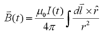
Where r is the vector from the source (dl) to the point at which we are evaluating the field. We can expect the displacement current term of Ampere's law,

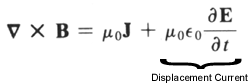
to affect our magnetic field, because we expect to see an electric field that changes with time. However, its contribution is scaled by the permittivity of free space, a factor ~10^-11. This means that in order for the displacement current to noticably affect the magnetic field, the change in electric field would have to be on the order of 10¹¹ V/m s.

This would entail a change in voltage in the circuit of Px10¹¹ V/s where P is the perimeter of the current loop. In the highly unrealistic case of a 10kV power source (much higher than we're likely to use), a loop perimeter of 0.1m (tiny) and a firing relay that switches in 1 milliseconds (unreasonably fast!!), the displacement current is then on the order of 1 Amp, but we are expecting power supply currents possibly as high as ~10000 Amps initially, making the displacement current contribution to B inconsequential.

Therefore, to get a value for B(t), we break the Biot-Savart integral up into four parts - the two rails, the slug, and the connection opposite the slug which we will approximate as a fixed armature across the rails. In reality, this connection will consist of the power source, the firing relay, and the connecting wires. Our assumption is that the field contribution of this portion of the circuit can, in fact, be manipulated to be very similar to a direct connection across the rails.

The direction of the magnetic field vector depends on which direction the current flows through the loop. For convenience, we'll assume that the current moves counter-clockwise. By the right-hand rule, the magnetic field is in the positive z direction, "up".

The magnetic field at some point, P, induced by current flowing through a straight wire can be derived analytically. A succinct example of this derivation is given in Griffiths, chapter 5, example 5. The following figure is taken from this example.

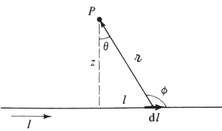
The end result is that

where z is the shortest distance from P to the wire, theta1 and theta2 are the initial and final angles between z and r. We will approximate the railgun as four straight wire field contributions summed together.

For the first rail:

z = y
sin(theta1) = -(L - x) / sqrt((L - x)2 + y2)
sin(theta2) = x / sqrt(x2 + y2)

z = (W - y)
sin(theta1) = x  / sqrt(x2 + (W - y)2)
sin(theta2) = -(L - x) / sqrt((L - x)2 + (W - y)2)

z = (L - x)
sin(theta1) = (W - y) / sqrt((W - y)2 + (L - x)2)
sin(theta2) = y / sqrt(y2 +  (L - x)2)

z = x
sin(theta1) = -y / sqrt(x2 + y2)
sin(theta2) = (W - y) / sqrt(x2 + (W - y)2)

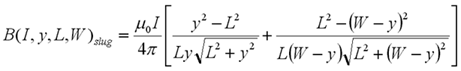
Oops, screwed that equation graphic up bad. It's all wrong, but the general form is right. it's B(I,x,y,L,W)|slug = (mu_oI/4pi)[f(L,W,x,y)]

2) Inductive EMF in Current Loop

Faraday's law tells us that when we have a changing magnetic field, we have an induced electric field.

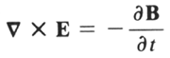
We take Faraday's law and act upon it with the curl theorem of vector calculus,

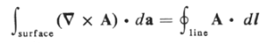
to achieve the following relation for the induced EMF, epsilon:

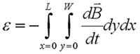
Again, this has been done analytically with Mathematica. [NOTE: Our initial railgun derivation used a slightly different form for epsilon, Griffiths 7.13. This is basically the same equation except the time derivative is pulled outside the integral because the magnetic field is assumed to be constant in time. This is obviously not the case for the railgun, and therefore the original derivation was incorrect.]

3) Ohm's Law

The induced EMF, calculated in section 3 above, opposes the power source voltage and therefore decreases the circuit current via Ohm's Law:

Where R is the circuit resistance. We'll assume that the resistance is constant with time, and we'll hope that it is very small. For this derevation, we will also assume that the power supply is a capacitor. This leads to the canonical form for I(t):

The capacitance of a capacitor is given by

where q is the amount of charge on the capacitor and V is the voltage across the capacitor. The charge at any time is given by

Now we can write the current like this:

Now we can take the derivative of this equation with respect to t to get a differential equation of I.

Some thought needs to be given to bounday conditions here, since the factor of q₀/RC has disappeared.

4) The Lorentz Force

The current in the loop flowing through magnetic field calculated in part 1 generates a Lorentz force outwards on the loop. The Lorentz force on the slug can be calculated analytically (Griffiths 5.17):

The magnetic field in this equation is given the subscript 'slug' because we are only interested in the field at the slug. This is the only part of the field that contributes to the Lorentz force on the projectile itself.

To calculate this magnetic field, we'll use the same technique and assumptions used in part 1. However, we can simplify the analysis here a bit since we'll always be at x=L. Also, the contribution to the field from the slug itself can be ignored.

Intuitively, if the slug were just a piece of straight wire, no amount of current through that wire would cause it to move anywhere in the absence of external fields. In the actual system, where the slug is under the influence of large magnetic fields, it can still be shown that the slug current won't move the slug. It's a simple matter of momentum conservation. If the slug moves itself, then momentum has been created from nothing.

Since the magnetic field is uniformly vertical and the slug lies horizontally on the rails, it is clear that the direction of the force will be horizontal and perpendicular to the slug, i.e. in the x direction. The cross product coveniently drops out, and all vectors becomes scalars with the exception of an x-hat at the end.

This is also equal to the mass of the slug times the acceleration of the slug (Newton's 2nd law of motion, F=ma). The acceleration of the slug can be written as the second time derivative of L, leading to this equation:

This equation can be solved for the current:

5) Differential Equation of Motion

The results from parts 4 and 5 can be combined to replace all instances of I(t) and I'(t) and leave a differential equation in terms of L(t), L'(t), L''(t), etc. (slug position, velocity, acceleration, etc)

It is hoped that Mathematica will be able to solve this differential equation to give an analytical form of the equations of motion for the slug in terms of physical variables like the mass of the slug, rail separation, and capacitance.

This will represent the end of the theory effort for the railgun and we will then proceed to design considerations and begin construction. (assuming, of course, that the numbers don't indicate that we require 1000 Farads of capacitance or one million volts or something.)