Abstract: The current focus of this research is the magnetic suspension of an elongated cylindrical beam; topics include the design and implementation of noncontact actuators, noncontact sensors, and the controller. Different actuators have been designed and built to generate different magnetic field patterns. The performance of the actuators, including the relations between forces versus positions and current inputs, are calculated and experimentally tested on our designed testing stage. The design rules and formulas of the tube suspension actuators are also derived and categorized for future usage. Different noncontact position sensors are designed and built based on the concept of differential transformers. The 3-pole sensor is an optimized design to reduce the cross coupling of the x and y positions. The sensor is excited by three primary coils at 10 kHz, and x, y positions are interpreted by the output of three secondary coils. A one-actuator-one-sensor setup had been made, and has successfully suspend the tube using a lead compensator. Further research will be done to study the suspension control and vibration control of the cylindrical beam by multiple actuators and multiple sensors.
 
 

1. Introduction

Many industrial operations center on the processing of an elongated element moving axially through successive functional stations. Examples include steel rolling, plastic film production, paper production, coating, and printing, and the coating and painting of materials such as plastic and metal. In these processes it may be advantageous to be able to handle the product without directly touching it. The objective of this research is to establish general theory for electric and magnetic suspensions applicable to noncontact processing. The experimental demonstration will mainly focus on the magnetic suspension of a cylindrical beam in this research.

Some researchers have looked at the control of magnetic suspensions of flexible structures for noncontact processing [1][2][3][4][5]. However, none of the above references have properly integrated the analysis of the distributed modes of the levitated body with novel control structures to stabilize these modes. In the field of flexible structure control, there has been significant work in the area for space applications[6][7][8]. However, there is a fundamental difference between their work and this research, since in the noncontact processing, it is not feasible to add damping material to the structure, or locate actuators and sensors within the structure in order to gain control of the structural modes.

The experimental setup is designed to be a scaled down model of a real operating center. The size of the tube is selected to be 6.35 mm (0.25 in) in diameter, 1.14 mm (0.045 in) in wall thickness, and 3 m (10 ft) in length. The prototypes of actuators and sensors are designed to suspend this tube. In practice, we chose the inside diameters of both actuators and sensors to be 12.7mm (0.5 in) to allow sufficient air gap for experimental purposes. The 3 mm (0.125 in) air gap is considered relatively large compared with commercial electromagnetic actuators, such as motors, with the same dimensions.
 
 

2. Actuator Design and Test

In general, the design of a magnetic actuator should include the following issues:

1. Magnetic saturation ( saturation of the suspended object, saturation of the actuator back iron )
2. Required forces ( the maximum forces can be calculated by assuming that the suspended object is saturated )
3. Heat transfer ( one of the common factors that limits the actuator performances )
4. Actuator size
5. Air gap ( generally, magnetic force is proportional to the inverse of air gap squared )
6. Air gap compared to the size of the suspended object
7. Current source ( required voltage, required current, electronics for current control )
8. Bandwidth ( current controller, magnetic diffusion )
9. Force change versus position change ( cannot be stable by Earnshaw’s theorem)
10. Linearity with current
11. Force directions (0.5-D, 1-D, 2-D), Torque directions
12. Force coupling between x, y directions
13. Power efficiency ( power loss in coil resistance, power loss in power amplifiers )
14. Manufacturing ( difficulties of coil winding, laminations or ferrite cutting )

Figure 1: Two different actuator designs: From left to right, Dipole-Quadrapole actuator, and the Four-U-Core actuator.
 

2.1 Dipole-Quadrapole Actuator: The first design of the actuator is the "dipole-quadrapole" actuator. It has 3 current inputs, and generates 3 different magnetic field patterns that include 1 dipole field and 2 quadrapole fields. The force will be generated by the combination of these three fields.  The schematic field distribution is shown in Figure 2.
 

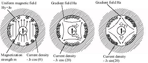
Figure 2: The magnetic field patterns of the dipole-quadrapole actuator: left one shows the dipole field, middle one shows the quadrapole w.r.t. force fx, and right one shows the quadrapole field w.r.t. force fy
 

2.1.1 Theory: The dipole-quadrapole actuator has 3 inputs: 1 dipole current input I₀ and 2 quadrapole current inputs I₁ and I₂. The current density amplitude J₀, J₁ and J₂ are corresponding to the current inputs I₀, I₁, and I₂. The actuator keeps dipole current I₀ constant, and changes I₁ and I₂ to control the forces Fx and Fy respectively. The assumptions are: (1) the tube inside the actuator is small enough such that it won’t affect the field distribution, (2) the field is considered to be 2 dimensional only. By the formula of Kelvin magnetization force density [9], the force density is:

The force generated by the actuator can then be obtained as

And r is the inside radius of the actuator. Under the previous assumption, this analytical result shows the properties that Fx and Fy will be de-coupled, and Fx and Fy will be neutral with respect to position change.
 

2.1.2 Matlab Simulation: The Matlab simulation is based on the analytical solution of the Maxwell equations. This simulation doesn’t neglect the existence of the tube. Commercial Finite Element Software can also be used to predict the force, however, using Matlab makes it faster to change dimensions and variables such as current inputs and tube positions. The simulation assumptions are: (1) the field is considered to be 2 dimensional only, (2) the magnetic scalar potential between the pole faces are assumed linear. We first solve the Laplacian Equation to get the magnetic field distribution of the air [11].

The force distribution can then be calculated by method of Maxwell Tensor [12]. And then we integrate the force distribution around the tube to obtain forces Fx and Fy. With 0.3A dipole current I₀, the formulas of the forces are obtained as the following

Fx (N) = 1.4 I₁ (A) + 0.3 x (mm)

Fy (N) = 1.4 I₂ (A) + 0.3 y (mm)

 
2.1.3 Testing Result: An actuator is built based on the dipole-quadrapole model. Instead of using a round cavity, we use 12 poles for the actuator, and the coils are wound in between the poles. We use an analog Proportional-Integral controller with power amplifier to reach the bandwidth 10,000 rad/s, the circuit design is modified from the previous research done in our lab [10]. A testing stand is also built to test the forces of the actuator generated while changing current inputs and positions of the tube. The testing result with 0.3A dipole current is further analyzed and the forces measured as the following:

Fx (N) = 0.9 I₁ (A) + 0.1 x (mm)

Fy (N) = 1.3 I₂ (A) + 1.1 y (mm)
 
We can see the differences between the dipole-quadrapole field theory, Matlab simulation and experimental results. The differences are basically from the assumptions that we made in the analysis. Other possible reasons could be the deformation of the tube and the saturation of some poles.
 

2.1.4 Pros and Cons: The advantages of the dipole-quadrapole actuator are that:

1. It is designed based on field pattern, instead of magnetic circuit approximation, it works better for small diameter tubes. When small tubes are being used, the assumption is closer to the real situation, and the nice properties of dipole-quadrapole actuator will show up.
2. The actuator is almost neutral in the x direction, it is easier to control.
3. The forces in x and y directions are de-coupled.
4. The forces are linear with currents.
5. The force will increase even when the tube is saturated, since the magnetic field tends to go through the tube.

1. Once the tube is attracted and in contact with the side-wall, it can not be released unless the dipole current is turned off.
2. It is difficult to wind the coil.

2.2.1 Theory: It is a simpler design, and proved to be more efficient than the dipole-quadrapole actuator in reality. Considering one independent U-Core electromagnet alone, the force applied on the tube from the U-Core electromagnet will be proportional to current squared divided by air gap squared. However, because the air gap is relatively large compared to the tube size, we’ll need to use Laplacian Equation to solve the magnetic field distribution generated by all four U-Core electromagnets to predict the force.
 

2.2.2 Matlab Simulation: Similarly, the Matlab simulation is done under the same assumptions as previously: (1) the field is considered to be 2 dimensional only, (2) the magnetic scalar potential between the pole faces are assumed linear. However, unlike the dipole-quadrapole actuator, the distance between pole faces in the 4-U-Core actuator is relatively large compared to the air gap. Hence the second assumption can easily fail, some adjustments of the simulation boundary conditions need to be done later.

The current inputs on each U-Core electromagnet are (I₀+I₁) and (I₀-I₁) for x direction electromagnets, and (I₀+I₂) and (I₀-I₂) for y direction electromagnets. I₀ is constant, I₁ controls the x direction force Fx, and I₂ controls the y direction force Fy. The simulation results with I₀ = 0.5A show that

Fx (N) = 11 I₁ (A) + 1.0 x (mm)

Fy (N) = 11 I₂ (A) + 1.0 y (mm)

 
2.2.3 Testing Result: The 4-U-Core actuator is designed and built. Note that the back iron of the actuator is made thick to prevent the saturation of the actuator. Since only uni-directional current is required, we use power FET’s to drive the actuator instead of expensive power amplifiers. The circuit design with quick fly-back circuit is modified from the previous research done in our lab [13]. The testing result for I₀ = 0.5A is further analyzed and the forces can be shown as:

Fx (N) = 6.0 I₁ (A)

Fy (N) = 6.0 I₂ (A)

The large differences between the Matlab simulation and experimental results are basically from the second assumption that we made in the analysis. Since we assume linear scalar potential between the pole faces, we overestimate the force applied to the tube.
 

2.2.4 Pros and Cons:
The advantages of the 4-U-Core actuator are that:

1. The actuator is almost linear with current and with position.
2. The forces in x and y directions are de-coupled.
3. It is easy to manufacture.
4. It is more power efficient.

1. It will not be working with small diameter tubes or strings.
2. The force will not increase when the tube is saturated.

(1) Basically, the controller of the current source determines the bandwidth of the actuator. The bandwidth of magnetic diffusion of the suspended object is not of concern here since the required force here is small, and a certain skin depth is plenty to support the tube. However, the issue of skin depth should to be considered when the required force per unit volume is so large that the object will be saturated.

(2) By using power amplifiers or power FET’s to drive the electromagnet, there will be a major percentage or power loss in the circuits. If higher power efficiency is needed, we can use PWM method to reduce the power loss, however the tradeoff is that the bandwidth and accuracy of the power input will be sacrificed.

3. Sensor Design and Test

3.1 Overview of Sensor Operation: The ability to sense an object without contacting it is especially beneficial when the surface of the object is subject to change. Often, non-contact sensors require relatively small air gaps and surfaces which present a constant target for the sensor. Two major advantages of the sensor described herein are robustness with respect to surface finish, and the ability to have a large air gap. The sensor output depends on the position of the tube, the permeability of the tube, and the geometry of the sensor components.

Various design iterations have been made through the course of this research. The final design, shown in Figure 3, uses a differential flux measurement to determine the position of the tube, which passes through the center of the sensor. The primary coils drive a field which circulates through the air-gap in the center of the sensor, then back around through the laminate core. The path of the flux is dependent on the tube position, and the voltages across the secondary coils are in turn dependent on the flux passing through them. By reading the voltages across the secondary coils, the flux passing through them can be determined, and this information can be used to determine the position of the tube within the sensor.

Figure 3: The Sensor and the schematic drawing of the sensor operation

 
3.2 Operation: The primary coils are driven with a three-phase current at a frequency of 10kHz, each pole out of phase by 120^o from the neighboring poles. Because the poles are also arranged geometrically at 120^o intervals, the induced magnetic field is a travelling wave with the same frequency. A magnetic field at this frequency will only penetrate aluminum to about 0.85mm; the aluminum shielding in Figure 3 therefore guides the flux by not allowing it to escape the air-gap region without returning through a lamination pole. Similarly, aluminum plates are used to sandwich the sensor to reduce leakage fields in the out-of-paper direction.

The voltages across the secondary coils are varying sinusoidally at 10kHz; as the tube changes position, the amplitude and phase of these signals will change. The tube position has a greater effect on the magnitude of the signal than the phase, so only the amplitude is used to predict the tube position. Although this means some of the information is not used, there are still three signals used to find two position measurements, which help reduce error. Each signals is demodulated to retrieve the information; this entails multiplying the signal by the sign of itself - synchronously rectifying it. By demodulating the voltage signal against itself and low-pass filtering the result, a constant voltage is obtained which corresponds to the amplitude of the original signal.

The three voltages from the three secondary coils can now be used to determine the position of the tube. An analysis of the fields in the sensor will give equations relating the output voltages to the tube position. By inverting these equations, the tube position can be solved for in terms of the output voltages. By combining the voltages in this way, two additional output voltages are obtained, one that corresponds to the tube position in the x-direction, and another in the y-direction.
 

3.3 Construction: The majority of the parts used are made using a water jet machine, which uses a high pressure stream of water mixed with abrasive grit to cut through materials. Although the precision of the machine is not as high as traditional machining, the speed with which complex 2-dimensional shapes can be cut makes it invaluable. The lamination sections, inner shielding sections and outer shielding ring are cut using the water jet; total cutting time for one sensor is just over an hour.

Silicon iron is used as the lamination material; 0.007" sheets are glued together using thermally conductive epoxy. The primary coils are 26 gauge wire with 35 turns; the secondary coils are 34 gauge wire with 350 turns. The shielding, both inside the sensor and outside, is cut from ½" aluminum stock.
 

3.4 Analysis and Testing: The sensor is modelled analytically to predict the output voltages across the secondary coils as the tube moves. Because of the asymmetry of the fields when the sensor is off center, the system is modelled using an analogous magnetic circuit, as seen in Figure 4.
 

Figure 4: Magnetic circuit approximation of the sensor analysis
 

In this type of analysis, the flux is modelled as a current, the Ampere-turns of the primary coils as voltage sources, and the flux paths(or reluctances) as resistances. Solving this circuit using traditional circuit analysis techniques results in equations for the voltages across the terminals in terms of the tube position. To test the accuracy of the analysis, the sensor is set up on an x-z table, with the tube passing through the center. With the x- and y-output voltages plotted against each other on an oscilloscope set on infinite persistence, the x-z table is moved in a 1mm grid throughout the range of the sensor. (The plane defined by x and y in the sensor frame of reference is the same plane as defined by x and z in the testing table frame of reference.)  If the sensor were perfectly linear, the output on the scope would be a linear grid, truncated by the circular shape of the interior of the sensor. In the center of the range, the actual output is similar to the ideal, but as the edge is approached the grid loses linearity. Figure 5 shows the experimental output from the sensor, alongside the theoretical output. The analytical output matches the experimental closely in the middle range, but diverges as the tube approaches the edge of the sensing range. Although the output is not perfect, because the sensor is used to null the tube position, it is sufficient to stabilize the tube under closed-loop control.
 

Figure 5: Experimental Output vs. Theoretical Output - Each line is made from plotting the x voltage vs. y voltage as the tube is moved in a 1mm grid.

The output electronic circuit has adjustable gain; currently it is set at 2 volts per millimeter, with the total usable range a 6mm diameter circle. At this setting, the signal noise is plus/minus 100millivolts, and most of that is from the low-pass filter which converts the 10kHz signal into a constant signal. A higher order filter would give a larger attenuation of the sinusoidal signal, but would also add phase lag to the system, making it more difficult to stabilize.
 
 

4. Feedback Control

With the testing results of the sensor and actuator, the tube dynamics can be modeled, and then the tube can be suspended by feedback control. Notice that the tube will vibrate along certain modes; these modes have nodes, where there is no motion. Placing a sensor at a node will leave that mode unobservable, while placing an actuator there will leave the mode uncontrollable. Additionally, the actuator applies a force at a position near to, but not exactly at the position being sensed. This noncollocation means that any mode with a period smaller than the noncollocation distance will not be controllable.

The tube dynamics are modeled by a Finite Element Method using the Bernoulli Beam Elements. The modeling is implemented by Matlab, such that the dynamics of the actuator can be included in the model easily.  The control algorithm can also be designed and simulated on computer using Matlab. A testing stage is built to suspend a short tube using one actuator and one sensor, as shown in Figure 6. The tube is simply supported at one end by a flexure, and suspended at the other end.
 

Figure 6: The testing stage for rigid body magnetic suspension. The left part shows the flexure, and the right part shows the sensor and actuator

A lead compensator is designed such that the system is stable with a bandwidth of 50Hz, which is well below the first mode at 100Hz. The closed-loop frequency response in y-direction of the system is shown in Figure 7, dashed line shows the nominal frequency response, and solid line shows the measured frequency response. Note that the input is required position, and the output is the measured position. In the experiment, although the system is stable, the first mode vibration is considerably obvious.
 

Figure 7: Closed-loop Bode Plot of the system, input is y position reference input, output is y position sensor output

5. Conclusion

This research has accomplished the noncontact actuator design, noncontact sensor design, and rigid body magnetic suspension of the tube. Further research will be done in the area of multi-sensor and multi-actuator control of magnetic suspension and vibration suppression. We will be consider the following issues as our next step:

1. Optimization of the sensor/actuator positioning ( observability/controllability )
2. Novel controller design for flexible structures
3. Robustness of the controller design, considering modeling error, sensor noise and actuator disturbances

Acknowledgments

The authors express their gratitude to the NSF for funding this research, with Grant award number: DMI-9700973.
 

 
References

[1] Y. Oshinoya, et al., "Electro-magnetic Levitation Control of an Elastic Plate," International Conference on Maglev, 1989.
[2] H. Hayashiya, et al., "Elastic Steel Plate for Steel Making Process," ICEE 1995.
[3] H. Osabe, et al., "The Effect on the Multipolar Electromagnet for the Levitation of Thin Iron Plate," MAGLEV 1995.
[4] K. Fujusake, et al., "Electromagnets Application to Thin Steel Plate," 1996 (no source listed on paper).
[5] S. Mori, et al., "Research on Levitation Magnets Switching for Magnetically levitated Conveyance System," LDIA 1995, nagasaki, Japan.
[6] ASME, "Active Control of Vibration and Noise," International Mechanical Engineering Congress and Exposition 1994.
[7] W. Gawronski, "Balanced Control of Flexible Structures," Springer-Verlag London Limited 1996.
[8] T.T. Hyde, et al., "Active Vibration Isolation for Precision Space Structures," MIT 1996
[9] J.R. Melcher, "Continuum Electromechanics," The MIT Press 1981, pp.3.8.
[10] Williams, "Precision Six Degree of Freedom Magnetically-Levitated Photolithography Stage," MIT, pp.157-165.
[11] H.A. Haus, et al., "Electromagnetic Fields and Energy," Prentice-Hall 1989.
[12] H.H. Woodson, et al., "Electromechanical Dynamics, Part II: Fields, Forces, and Motion," Robert E. Krieger Publishing 1968, Chapter 8.
[13] T. Poovey, et al., "A Kinematically Coupled Magnetic Bearing Calibration Fixture," Precision Engineerging: Journal of the American Society for Precision Engineering, Vol. 16, No. 2, April 1994.