Nature in a spinning water tank

Instructions: Please maximize your browser. You will need the ability to play wmv and mpegs, preferably embedded videos through plugins in your browser. This page has been tested on IE7/WMP (XP), and Firefox/mplayer (linux). Please turn on sound and speakers, it will enhance your experience.

Summary

We present a vision system for tracking rotating fluids and use it in a laboratory study of geophysical flows. Our system observes fluid-flow and constrains a numerical model with observations using an ensemble filter. A novel sampling scheme using a mixture of time snapshots and boundary condition perturbations allows us to track very high-dimensional states in realtime.
To the best of our knowledge, the demonstrated realtime system has not hitherto been reported. The economy and repeatability of experiments and the direct connections to planetary circulation implies that this our framework can be a perfect engine for interdisciplinary research in learning, vision, graphics and computational science to understand fluids. The success of our tracking algorithm suggests that a general method to overcome sampling limitations for tracking with monte-carlo methods may be at hand.

Why Rotating Fluids

Our oceans and atmosphere are perhaps the most visible example of rotating fluids, when viewed within the rotating frame. The figure on your left is a high-resolution image of upper-air analysis centered around the north-pole. The rich structure you see in terms of highs and lows on the pressure contours will evolve dynamically. By clicking here you will be able to see an animation of the GFS forecast from a nice interface created at the University of Wyoming. Along with the 500mb heights, you will also see wind-speed and temperature overlayed in color.

The Differentially-heated rotating annulus

The dynamical properties of the large-scale atmospheric circulation can be understood by studying the differentially-heated rotating annulus experiment. When a spinning annulus' center is cooled relative to a warm periphery, the water near the center becomes dense and sinks. Warm waters from the periphery move in to replenish thus setting up a radially overturning circulation. Instability due to strong thermal gradients and rotation rates produces eddies and jets like the mid-latitude atmosphere.
In the video below, you see platform with a water-tank. This platform is rotating and the camera is in the rotating frame (that is why the person's hand rotates later in the video). Ice in a can is cooling the core in the middle whilst the periphery of the water-tank is forced by ambient room temperature. Notice how the dye (red is warm, green is cold) evolves. The rich structure so formed arises from dynamics similar to the large-scale problem.

Overview of Coupled Physical-Numerical System

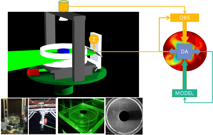
We built an automated observatory for rotating fluids and study the differentially heated rotating annulus. By observatory we mean three things: A physical simulation as you see above from which observations are gathered automatically, a numerical simulation, and algorithms that constrain models with observations. All three embody the concept of an observatory as a single coupled system with which to understand the fluid, and the system functions in realtime.

The physical component of the coupled system, as seen in the figures and will be evident in videos to follow, consists of a fluid embedded with neutrally bouyant particles, a laser, a robotic arm to illuminate particles in a plane, a camera to watch them move, all of which sit on a turntable spinning with periods between 3-8 seconds.

The computational component is highly distributed and heterogenous. This subsystem produces measurements (velocities via optic flow), model states (via numerical simulation), and estimates of model-states (and their uncertainties) conditioned by observations. We have achieved realtime performance by using many tricks: Nonuniform discretization, spatial domain decomposition, spectral decomposition, and something we think is new; a monte-carlo (ensemble or particle) tracking algorithm with novel way to represent and sample from the distribution of model-state's uncertainty.

Tracking Rotating Fluids in Realtime Using Snapshots

S. Ravela, J. Marshall, C. Hill, A. Wong and S. Stransky, A Realtime Observatory for Laboratory Simulation of Planetary Flows, Experiments in Fluids, 2009

Videos depicting the observatory can be viewed through the player-object embedded in the left half of this web-page, below. A commentary accompanies the videos on their right.
If you cannot see any video in about a minute, kindly click on the file names (active links) at the begining of text descriptions to see the corresponding video.

(1) File Apparatus.wmv. This video shows the system -- the rig, robotic-arm with mirror, chiller, camera, and FORJ. Once the fluid enters solid body rotation, the chiller is turned on, which is marked by a change in ambient acoustics in the video. A temperature value at a point in the interior of the cold-core is displayed on the LCD panel. The laser is turned on once the core cools to approximately 0C and the video ends.

	(2) File Obs.wmv. This video shows the camera's view of illluminated particles at some layer of the fluid in the rotating frame (after circulation has set in). Particles can be observed (albiet at low resolution) to move with the flow in eddies and vortices. The green lines (arrows) indicate realtime velocity vectors overlayed on the video. It must be noted that the velocity vectors can be noisy, especially at the boundaries of the interior and shadow regions of the annulus. The yellow lines overlayed in the last quarter of the video show the (unconstrained) model vectors also in realtime. Both vectors are plotted to the same scale (~2cm/s).
	(3) File VolumeObs.wmv. This video shows the mirror moving through the volume taking measurements at five layers. Each scan takes approximately 5 seconds to complete.
	(4) File Assimilate.wmv. This video shows the model velocities being constrained by observed velocities, depicted for a single ensemble member at a single horizontal layer of the fluid (but estimation itself is over the volume, see paper). The video shows model velocity vectors on the right as the model spins up (00:00 - 00:04s of video time) to roughly 200s of simulation. The first set of observations are encountered, vectors flash on the left panel of video, and the model field immediately adjusts. At the next time step, observations are no longer available, and the panel on the left becomes "blank." As time progresses, forecast model velocities are shown on the right and updated every second of simulation time. After 10-model seconds (00:10s mark on video time), new observations are available, and the model adjusts itself again. In this way, the forecast, assimilate cycle continues. Over time, one can observe that the model vectors become consistent with the observations. Notice that these adjustments are robust in the presence of observation noise, and that the model fills in a circulation, where one is not present in the observations, in a manner consistent with the large-scale circulation. By the end of the estimation sequence, the model is nicely registered to observations. Note again that only one slice of the 3D volume is being shown. The whole volume is estimated.
	(5) Files: TempTankTopPol.wmv and TempTankTopCart.wmv. These videos show open loop simulations of the model, depicting the temperature field at the top of the tank in polar (left) and cartesian (right) coordinates. Note that these videos are synchronized relative to one another, but not to wall-clock time.Nevertheless, they give a sense of the nature of flows produced numerically for the rotating annulus experiment described in the paper.

Broader Impact

***UNDER CONSTRUCTION***

Fluid Understanding: Effective Parameterizations of Models

When the numerical system tracks the physical system in realtime, we can augment reality with numerical metrics and features that cannot be observed. For example, the distribution and evolution of effective thermal diffusivity can be systematically and economically studied to improve diffusivity parametrization of ocean circulation models.

Interactive Fluid Visualization

An associated problem is to visualize the coupled system's fluid state or properties derived from the state in 3D, in realtime. This has obvious connections to graphics.

Algorithms for Distributed Lagrangian Measurement

Active Observer Design

Eulerian measurements in the real ocean or atmposphere are only possible as vertically integrated or surface measurements using satellites. We may, on the other hand, want insitu measurements in a number of situations. For example, using a numerical system that tracks the physical system, we can release an artificial tracer (dye) into the numerical fluid. We can then devise planning and control algorithms for autonomous underwater vehicles to track the evolution of the numerical dye and deploy these strategies in the real-world. Our algorithms will have to account for all the uncertainties that we might expect from imperfect knowledge of the true physical system, erroneous models, and tracking errors, which would be valuable for building robust real-world observers.

Data Assimilation: Nonlinearity, Dimensionality and Uncertainty

Algorithms for constraining a numerical model with observations are fundamental to ocean state estimation and numerical weather prediction. In these applications, predictions are made using general circulation models (GCMs). Even a perfectly calibrated and parametrized GCM will not predict the atmosphere (say) perfectly, when initial conditions are uncertain. Estimating model-states and their uncertainties is thus the primary means to constrain a GCM.

Tracking the laboratory flow is convenient and useful for the state estimation problem in the large-scale because repeatable experiments with real data can be performed using far simpler logistics than the operational setting. Further, key challenges in the large-scale problem must also be addressed in the laboratory setting: (a) Nonlinearity --- the laboratory analog is nonlinear and the numerical model is the same used in planetary simulations. (b) Dimensionality --- the size of the state of the numerical model is of the same order as planetary simulations. (c) Uncertainty --- the initial conditions are unknown, and the model is imperfect relative to the physical system. (d) Realtime --- forecasts must be produced in better than realtime. Solutions to these problems can accelerate operational acceptance of new methods (as well as inform estimation for many other coupled numerical-physical systems).