Project 1: Modeling of the Ocean Circulation
State-of-the-art, fully realistic numerical ocean general circulation models (OGCM) are used to simulate and predict the time evolution of the field of currents, temperature and salinity at different depths. Examples for full oceanic basins; energetic current systems such as the Gulf Stream; and semi-enclosed basins are given below.
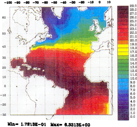
1a) The Atlantic Ocean
Fig. 1 Sea surface temperature (C): El model mean
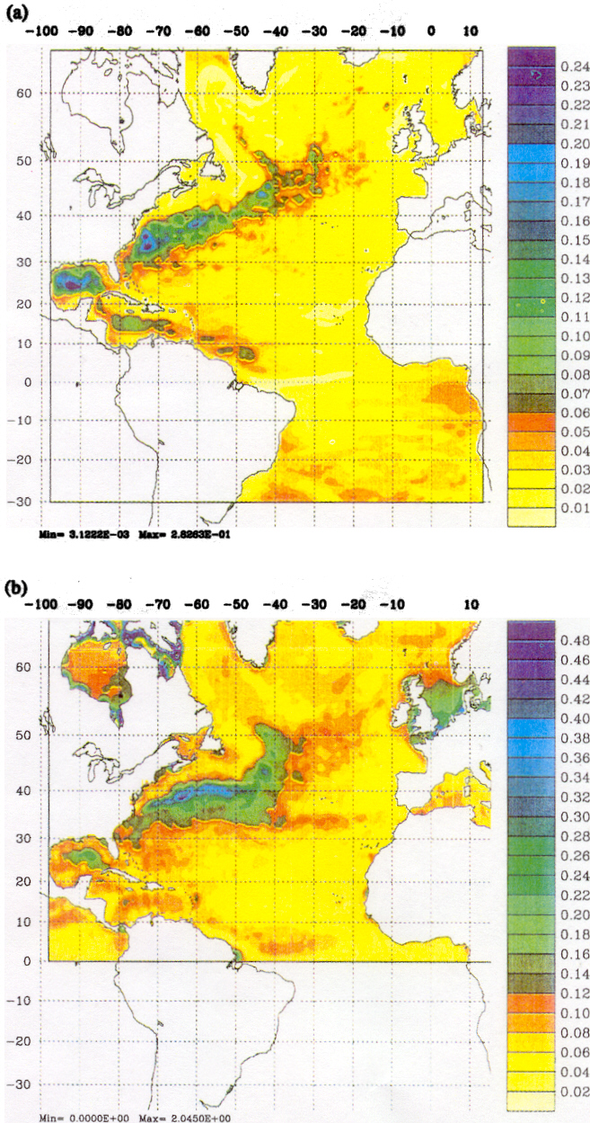
Fig. 2 Sea surface height variability (m2): (a) E6 and (b) Topex (from Gregg Jacobs, NRL).
1b) The Gulf Stream System

Fig. 3 Composite remote sensing/in-situ data set and the locations of the Gulf Stream North Wall and rings for June 13, 1988. Key: 200-m isobath, white; Geosat groundtracks and dynamic topography, white; AXBT/CTD locations, yellow/purple symbols; Gulf Stream North Wall and ring edges, black; ring centers, black/white cross. AXBT/CTD temperature at 200 m: 12.50ºC plus; 12.50-15.0ºC, star; 15.0-17.50ºC, circle; >17.50ºC, square.
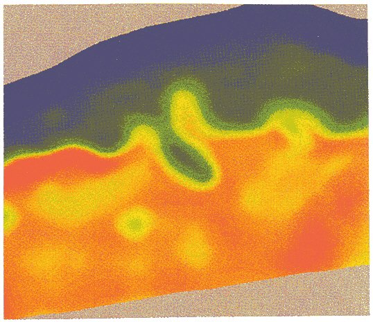
Fig. 4 Density Field at 200 m depth at day 62 of the hindcast experiment starting on May 4, 1988, and ending on December 28, 1988, with bi-weekly assimilations of OTIS 3.0 fields.

Fig. 5 - Top panel: no assimilation. Bottom panel: assimilation of the local datasets (current and temperature measurements at the localized arrays of Fig. 11) 42 days from the beginning of the experiment. Significant differences are evident in the mesoscale eddy field.
1c) The Eastern Mediterranean
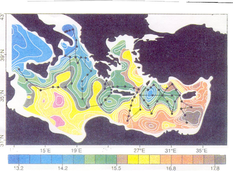
Figure 6 - The Eastern Mediterranean basin. Network of the January 1995 survey of the R/V Meteor (Germany) superimposed on a map of the temperature at 125m depth throughout the basin. Large dots indicate hydropgraphic and tracer stations, where the physical, chemical, and biological parameters were measured. The two diamond-shaped regions in the lower right section mark the area of intensive field work covered by successive surveys in February, March, and April 1995.
1d) The Black Sea
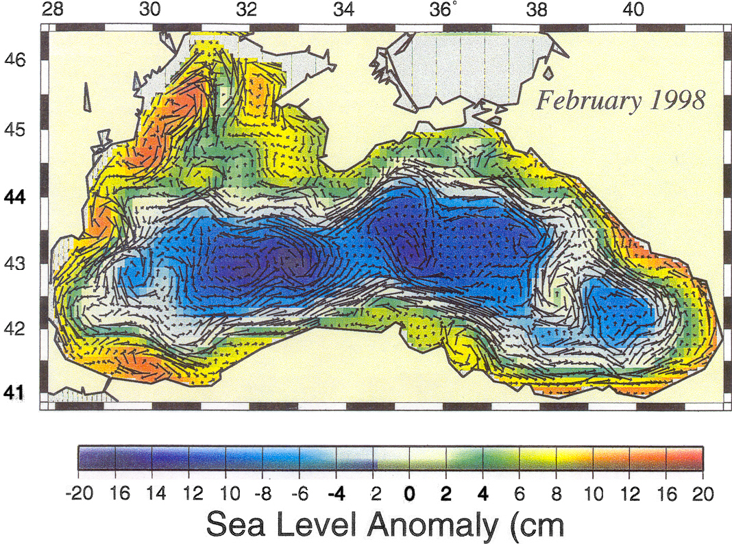
Fig. 7 The upper layer circulation pattern for February 1998 shown as an example for the winter horizontal flow structure. It is derived by assimiliation of the Topex-Poseidon and ERS II altimer data into a 1.5 layer reduced-gravity model. The background colors colors show the corresponding sea level anomaly pattern given by the altimeter data.