Basic
Concepts
Here I explain some issues that arise
when the multiple particle tracking is performed on heterogeneous systems.
I give conceptual examples to illustrate limitations and show how the
latter can be overcome using some realistic assumptions.
Calculating
the msd

To calculate the mean-squared displacement
from a trajectory, this trajectory must be divided into displacements.
If we go back to the trajectory list I was showing in the previous section ,
we extract from trajectory 1 (which lasts from time j=0
to j=4) the following displacements
at a lag time of 1:
,
we extract from trajectory 1 (which lasts from time j=0
to j=4) the following displacements
at a lag time of 1:
At a lag time of 2 we can extract these displacements:
We can repeat this calculation for all the trajectories, and we can perform this at various lag time. Note that these displacements are overlapping on the same trajectory, meaning that they are not statistically independent. This can become an issue when using quadratic formula of the displacements in estimators and it can be solved by performing a block-average of the displacements. I don't discuss this particular issue in this tutorial, but you can refer to the original article on block-average by Flyvbjerg & Petersen (1989), or find a detailed explanation for the particle tracking case in the article by Savin & Doyle (2007). Both articles are referenced here.
The general formula for the displacements is:
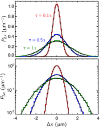
which is valid as long as the trajectory contains the times j and (j+τ). From a trajectory i of duration Ti, you can compute ni displacements, with ni = Ti+1-τ. The longer the trajectory and the smaller τ are, the more displacements can be extracted (and the more precise will be the estimate of the msd). For a given lag time, we obtain a list (or sample) of displacements coming from several trajectories. Ignoring the generating trajectory for each displacement, thus considering all displacements in the same sample, we can plot the distribution (or equivalently the histogram) of the displacements. This is called the van Hove correlation function and it is specified for a given lag time. I show an example of this distribution at 3 different lag times in the figure above (obtained for 0.5 μm-diameter spheres mixed in water). I was able to gather a lot of displacements in this experiment, so the distributions are nicely fitted by Gaussian distributions. The variance of this distribution is precisely the mean-squared displacement. It is a time average because the displacements were originated from various time along each trajectory, and an ensemble average because these displacements come from different trajectories. Repeating this calculation at several lag times, by building new displacements sample, and calculating the variance of the van Hove correlation function generated for each lag time, we can calculate msd(τ) as I did in the first section. As said before, for a given lag time, the more trajectories, and the longer they are, the more displacements the sample will contain. Consequently the ensemble mean-square displacement will be more precisely calculated.
| Δr10 = ( Δx10 = x11 -x10 , Δy10 = y11 -y10 ) |
| Δr11 = ( Δx11 = x12 -x11 , Δy11 = y12 -y11 ) |
| Δr12 = ( Δx12 = x13 -x12 , Δy12 = y13 -y12 ) |
| Δr13 = ( Δx13 = x14 -x13 , Δy13 = y14 -y13 ) |
At a lag time of 2 we can extract these displacements:
| Δr10 = ( Δx10 = x12 -x10 , Δy10 = y12 -y10 ) |
| Δr11 = ( Δx11 = x13 -x11 , Δy11 = y13 -y11 ) |
| Δr12 = ( Δx12 = x14 -x12 , Δy12 = y14 -y12 ) |
We can repeat this calculation for all the trajectories, and we can perform this at various lag time. Note that these displacements are overlapping on the same trajectory, meaning that they are not statistically independent. This can become an issue when using quadratic formula of the displacements in estimators and it can be solved by performing a block-average of the displacements. I don't discuss this particular issue in this tutorial, but you can refer to the original article on block-average by Flyvbjerg & Petersen (1989), or find a detailed explanation for the particle tracking case in the article by Savin & Doyle (2007). Both articles are referenced here
| Δrij(τ) = ( Δxij = xi(j+τ) - xij , Δyij = yi(j+τ) - yij ) |
which is valid as long as the trajectory contains the times j and (j+τ). From a trajectory i of duration Ti, you can compute ni displacements, with ni = Ti+1-τ. The longer the trajectory and the smaller τ are, the more displacements can be extracted (and the more precise will be the estimate of the msd). For a given lag time, we obtain a list (or sample) of displacements coming from several trajectories. Ignoring the generating trajectory for each displacement, thus considering all displacements in the same sample, we can plot the distribution (or equivalently the histogram) of the displacements. This is called the van Hove correlation function and it is specified for a given lag time. I show an example of this distribution at 3 different lag times in the figure above (obtained for 0.5 μm-diameter spheres mixed in water). I was able to gather a lot of displacements in this experiment, so the distributions are nicely fitted by Gaussian distributions. The variance of this distribution is precisely the mean-squared displacement. It is a time average because the displacements were originated from various time along each trajectory, and an ensemble average because these displacements come from different trajectories. Repeating this calculation at several lag times, by building new displacements sample, and calculating the variance of the van Hove correlation function generated for each lag time, we can calculate msd(τ) as I did in the first section. As said before, for a given lag time, the more trajectories, and the longer they are, the more displacements the sample will contain. Consequently the ensemble mean-square displacement will be more precisely calculated.
Particles
dynamics in heterogeneous systems - distribution of msd
Microrheology is often performed in
complex and heterogeneous systems. It is actually one of the main strength
of microrheology to be able to probe a material locally, at a length
scale that is below some material structural size. In that case, a particle
labeled k and fluctuating around
a given location in the material will have a certain dynamical signature,
quantified by its individual mean-squared displacement msdk(τ).
This individual dynamic results from the local mechanical property of
the material at the given location of the particle. Another particle
labeled l located at another
position in the material will exhibit another mean-squared displacement
msdl(τ),
and if the local mechanical property of the material at this location
is different from the one of the particle k,
then msdk ≠ msdl.
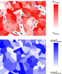
This is illustrated in the figure on the right, where I draw the schematic
of a heterogeneous material. Its mechanical property (called ν in
the figure) change with the location in the sample. I show the corresponding
map of msd for the particle dispersed in the sample. In order to calculate
msdk, we would divide
the trajectory k into a sample
of displacements, and then caculate the variance of this sample to have
a time average individual msd. We would repeat the same procedure with
all trajectories to then build a list of msd values, all calculated at
a given lag time. Each of these msd values represents the individual
dynamic of the beads in the material at various location, thus mapping
the corresponding spatial variations of material property.
Quantifying
heterogeneity
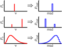
It is now clear that the distribution
(or histogram) of individual msd from multiple particle tracking can
be efficiently connected to the spatial distribution of the material
property of a sample. For example, if the material is strictly homogeneous,
all particles, no matter where they are in the material, will have the
same dynamics. Thus from each particle, the same van Hove correlation
function can be calculated and all mean-squared displacement will have
the same value such that plotting their histogram will show a unique
peak. Another example is a material that exhibits only two different
values of mechanical property. Then particles embedded in a region of
property 1 will all have an msd of value msd1, the ones in
region 2 will exhibit msd2. The distribution of msd will show
two peaks, thus efficiently mapping the distribution of material property.
We give an experimental realization of such a bimodal fluid in the next section.
This extends naturally to more general heterogeneous system with an arbitrary
spatial distribution of property, potentially mappable into a distribution
of individual particles' msd. This is illustrated schematically on the
figure on the right. Ideally, one would want to obtain this distribution
of msd. For statistical limitations that will become obvious in the next part,
this is not possible in most cases. Instead, we will calculate here moments
of this distribution. Hence, the mean of all the msd, if calculated efficiently,
can give information on the mean material property. This is what is done
in most one-point microrheology experiments, when measurements are performed
by averaging over all particles. But the second moment (that is, the
variance) of msd distribution gives a natural measure of its spread,
that is of how much the individual msd differ from one another. And this
can be related to the mechanical heterogeneity of the studied sample.
The trick now is to calculate these moments: the mean and variance of
the individual msd's, which are themselves the variances of the individual
van Hove correlation functions mentioned earlier.
Finite depth
of tracking
As we have seen in the first section,
particles can be tracked as long as they remain in focus. To be more
precise, they are trackable as long as their position in the z direction
(if (x,y) defines the imaging
plane) is within a certain interval called depth of tracking of the microscope.
If some particles exhibit large mean-squared displacement at a certain
lag time, they are likely to leave this interval within this particular
lag time and they will not be trackable for a longer time. On the other
hand if other particles are trapped and have a small msd, they will potentially
stay within the depth of tracking and will be trackable for a longer
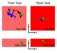
time. This effect is illustrated in the movie linked on the right hand
side. I have simulated Brownian motion in two Newtonian fluids: one with
a small viscosity (I call it "fast" in the movie) and one with
a large viscosity (the "slow" fluid). The particles are trackable
when they are in the tracking volume represented (top and side view)
in red on the movie. On the left-hand side of the movie, the particle
is moving in the "fast" fluid, and exhibit large amplitude
displacements. We see that the particle leaves and enters the tracking
depth several times, and every time is tracked as a new trajectory. On
the other hand, in the more viscous "slow" fluid on the right,
the particle does not exhibit large amplitude motion, and stay in the
tracking depth (or equivalently remains in the microscope focus) thus
producing only one trajectory. Comparing the value of the mean-squared
displacement (ideally in the z direction,
but this information is not usually measured; assuming isotropy of the
sample, the x- or y-msd
gives the same information) at a given lag time to the squared depth
of tracking of the microscope gives an idea of how important this effect
is. If the msd is bigger, the particle will leave the tracking depth
within this lag time giving only one or multiple short trajectory. If
the msd is smaller, the particle can be tracked for a longer time before
it leaves. Recall that if the trajectories are short, the msd is poorly
statistically resolved. And in some case there will be a lag time τ above
which the msd cannot be calculated since no displacement can be extracted
from a trajectory shorter than τ.
This is a fundamental limit that will be illustrated in the following section.
But for now we will assume that we are interested in sufficiently low
lag times so that all trajectories can produce some displacements to
calculate their corresponding msd.
The assumption
of constant density
The main consequence of the finite
depth of tracking is that it is not possible to build a meaningful distribution
of msd. From the example above we see that many more msd will be extracted
from a "fast" fluid, whereas few msd will be reported from
the "slow" fluid. This is the case even if the heterogeneous
fluid has as much "fast" region as "slow" regions.
The msd distribution will be biased towards large msd. This bias gets
more intricate when we recall that msd calculated from short trajectories
(which are, again, numerous in the "fast" fluid) are poorly
resolved, producing in the measured distribution a large statistical
spread for large msd. We will see that in the experimental example presented
in the next section.
So if the msd distribution is biased, how can we calculate anything unbiased
from it? It turns out that under the reasonable assumption of having
always a constant number of tracked particle in the volume of tracking,
the following quantities:
are (almost) unbiased estimators of the ensemble mean and ensemble variance of the individual msd distribution that correctly map the spatial distribution of the material. This means that:
are the mean and variance we are looking for. These quantities M1 and M2 are the weighted sample mean and variance of the sample of individual msd. The weight wi is proportional to Ti, the duration of the trajectory i, and the set of weight is normalized. Thus the shorter trajectories (which give the less precise msd's) weight less than the longer ones. But since they are more numerous, we will actually get an unbiased estimation. More precisely, the main argument is that the sum Σi Ti for trajectories located in a sub-region of material remains the same from one location to another, even if the material is heterogeneous. We illustrate in the next section how
these estimators perform on a canonical experimental system.
| M1 = Σi wi msdi |
| M2 = Σi wi (msdi - Σi wi msdi) 2 |
are (almost) unbiased estimators of the ensemble mean and ensemble variance of the individual msd distribution that correctly map the spatial distribution of the material. This means that:
| <M1>=<msd> |
| <M2>=<msd2> - <msd>2 |
are the mean and variance we are looking for. These quantities M1 and M2 are the weighted sample mean and variance of the sample of individual msd. The weight wi is proportional to Ti, the duration of the trajectory i, and the set of weight is normalized. Thus the shorter trajectories (which give the less precise msd's) weight less than the longer ones. But since they are more numerous, we will actually get an unbiased estimation. More precisely, the main argument is that the sum Σi Ti for trajectories located in a sub-region of material remains the same from one location to another, even if the material is heterogeneous. We illustrate in the next section