6.2.1 Shortest Paths From a Given Node to All Other Nodes [t(i, j) 2
0]
The first problem that we shall examine is that of finding the
shortest path between a given node and all other nodes on a given graph
G(N, A). It is assumed that all link lengths,  (i, j) are
nonnegative. (i, j) are
nonnegative.
The algorithm basically consists of beginning at the specified node s
(the "source" node) and then successively finding its closest, second
closest, third closest, and so on, node, one at a time, until all nodes
in the network have been exhausted. This procedure is aided by the use
of a two-entry label, (d(j), p(j)), for each node j.
In the evolution of the algorithm, each node can be in one of two
states:
- In the open state, when its label is still tentative; or
- In the closed state, when its label is permanent.
At any stage in the algorithm, the label entries for node j contain
the following:
- d(j) = length of the shortest path from s to j discovered so far
- p(j) = immediate predecessor node to j in the shortest path from s
to j discovered so far
Finally, we shall use the symbol k to indicate the most recent (i.e.,
the last) node to be closed and the dummy symbol "*" to indicate the
predecessor of the source node s.
The algorithm can now be described as follows:
First Shortest-Path Algorithm (Algorithm 6.1)
| STEP 1 |
To initialize the process set d(s) = O. p(s) = *; set d(j) =  ,
p(j) = -for all other nodes j ,
p(j) = -for all other nodes j  s; consider node s as closed and all
other nodes as open; set k = s (i.e., s is the last closed
node). s; consider node s as closed and all
other nodes as open; set k = s (i.e., s is the last closed
node). |
| STEP 2 |
To update the labels, examine all edges (k, j) out of the last
closed node; if node j is closed, go to the next edge; if node j is
open, set the first entry of its label to
d(j) = Min [d(j), d(k) + (k,i)] (6.1)
|
| STEP 3 |
To choose the next node to close, compare the d(j) parts of the
labels for all nodes that are in the open state. Choose the node with
the smallest d(j) as the next node to be closed. Suppose that this is
node i. |
| STEP 4 |
To find the predecessor node of the next node to be closed, i,
consider, one at a time, the edges (j, i) leading from closed nodes to i
until one is found such that
d(i) - {(a, i) = d(j)
Let this predecessor node be j*. Then set p(i) = j*.
|
| STEP 5 |
Now consider node i as a closed node. If all nodes in the graph are
closed, then stop; the procedure is finished. If there are still some
open nodes in the graph, set k = i and return to Step 2.
Upon termination of the algorithm, the d(j) part of the label of node
j indicates the length of the shortest path from s to j, while thep(j)
part indicates the predecessor node to j on this shortest path. By
tracing back the pa j) parts, it is easy to identify the shortest paths
between s and each of the nodes of G. |
Notes
- Ties in Step 3 can be broken arbitrarily [i.e., when two or more
nodes have equal d(j) and thus qualify as the next nodes to be closed,
choose one among them arbitrarily]. The same applies for ties for the
predecessor node in Step 4.
- The algorithm is easy to carry out in tableau form and especially
simple for computer implementation. When using the algorithm for manual
solutions, the procedure can be speeded up considerably by carrying out
Steps 2-4 almost simultaneously and virtually by inspection.
- The algorithm can also be used for finding the shortest path between
a source node and a specified terminal node. All that need be changed is
Step 5: termination now occurs as soon as the terminal node becomes
closed.
- The algorithm can be used with directed, undirected, or mixed
graphs, as long as (i, j)
 0 for all (i, j)
  A. A.
- This algorithm--or, more exactly, a minor variation of it--is
generally attributed to Dijkstra [DIJK 59], but many very similar
algorithms have been proposed by a number of researchers over the years.
Example 1
Consider the mixed graph shown in Figure 6.3 and suppose that the
source node is a. We wish to find the shortest paths from a to all the
other nodes.
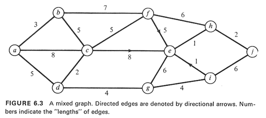
Solution
Figure 6.4a shows the labels on the nodes on completion of the first
pass over the five steps of the algorithm. Node b is the next node to be
closed; hence after this pass k = b. The two closed nodes up to this
point, a and b are indicated by a " +" next to their labels. These two
labels are thus permanent. [It is advisable in manual solutions to use a
special symbol (such as the " + ") to keep track of the closed
nodes.]
Figure 6.4b shows the status of the network's nodes after completion
of the second pass over the algorithm. The label of fhas changed, the
label of c remained unchanged (why?), dis the next closed node, and k =
dat the end of the pass.
Let us now trace in some detail what happens during the third pass.
The edges out of d to open nodes are (d, c) and (d, g). For c we
have
d(c) = Min [d(c), d(d) + 4(d, c)] = Min [8, 5 + 2] =
7
Thus, d(c) is changed from 8 to 7. We also change d(g) to 9 (from
). We now find that
| Min [d(c), d(e), d(f), d(g), d(h), d(i), d(j)] = | Min
[7, Do, 10, 9, ,
, ] |
| = 7 |
| = d(c) |
Thus, c will be closed next. The edges to c from closed nodes are (b,
c), (a, c), and (d, c). Checking, we find that d(c) -
(d, c) = 7 - 2 = 5 =
d(d). Therefore, we set p(c) = d (i.e., the predecessor of c is d).
Since there are still some open nodes, we set k = c to complete this
pass through the algorithm. The status of the graph at this point is
shown in Figure 6.4c.
Proceeding in the same way, and after six more passes, we finally
complete this work and reach the status shown in Figure 6.4d. The labels
now contain all necessary information about the shortest path from a to
every other node on the graph. For instance, the shortest path from a to
h is of length 15 and [working backward from p(h) to p(e) to p(i), etc.]
that shortest path is {a, d, g, i, e, A}. The tree that contains all the
shortest paths out of node a is now shown in Figure 6.5.
Trees like the one sh2own in Figure 6.5 are often referred to as
shortest-path trees.
|


