6.4.8 Probabilistic View of the Traveling Salesman Problem
Before completing this discussion, we state a very useful result on the
expected length of an optimum traveling salesman tour under a Euclidean
travel metric.
First, it is helpful to make the following observation. Suppose that a
traveling salesman tour has been drawn through n points all of which lie
in a given area A. Suppose now that this area is expanded uniformly m-fold.
This can be done by changing the coordinates (x, y) of every point in A to
( x, y).
The same traveling salesman tour through the same n points as
before will then be "stretched" in length to
times its earlier length,
for the simple reason that every linear segment in A has now been multiplied
by . Thus, quadrup ing, say, the area A in the
manner described above will
only double the length of the given traveling salesman tour. More generally,
we can state that a given traveling salesman tour varies in proportion to
the square root of the area in which it is contained. We have seen
equivalent results several times already in Chapter 3. x, y).
The same traveling salesman tour through the same n points as
before will then be "stretched" in length to
times its earlier length,
for the simple reason that every linear segment in A has now been multiplied
by . Thus, quadrup ing, say, the area A in the
manner described above will
only double the length of the given traveling salesman tour. More generally,
we can state that a given traveling salesman tour varies in proportion to
the square root of the area in which it is contained. We have seen
equivalent results several times already in Chapter 3.
With this observation, we now turn to the result of interest. Assume that
n points are randomly and independently dispersed over an area A with the
location of each point determined by a uniform distribution over A (i.e.,
each point is equally likely to be anywhere in A). Assume further that an
optimum traveling salesman tour has been drawn to cover the n points in
question, and let L(n, A) be the length of this optimum tour through the n
points in A. The following has then been shown to be true whenever the
assumptions above hold [BEAR 59]:
Theorem
Recently, K has been estimated as being approximately equal to 0.765
[STEI 78]. (An earlier set of simulation experiments had led to the estimate
K  0.75 [EILO 71].)
Like all limit theorems, the one above must be used carefully. For
instance,the value of n which is "large enough" (for the quantity 0.765
 to provide good approximations to the expected length of the optimal
traveling salesman tour) depends on the shape of the area in which the n
points are distributed uniformly. For "fairly compact and fairly convex"
areas (see also Section 3.7.1) it seems that surprisingly small values of
n may be adequate. For example, n = 15 or larger is quite adequate for
equilateral triangles, circles, or squares (see [EILO 71]).
to provide good approximations to the expected length of the optimal
traveling salesman tour) depends on the shape of the area in which the n
points are distributed uniformly. For "fairly compact and fairly convex"
areas (see also Section 3.7.1) it seems that surprisingly small values of
n may be adequate. For example, n = 15 or larger is quite adequate for
equilateral triangles, circles, or squares (see [EILO 71]).
While the proof of the limit theorem above is difficult, it is quite easy
to devise fairly intuitive arguments that lead to results of the form K
[EILO 71]. One of our homework problems develops such an argument, which
also contains some of the key characteristics of the formal proof of the
theorem.
The approximation formula 0.765
is a very useful one for:
| 1. | Preliminary planning of urban collection and delivery
systems (i.e., for "sizing up" the requirements for vehicle fleets,
estimating the number of points that can be served with given resources, etc.)
| | 2. | Assessing when a solution to a TSP obtained through some
heuristic approach is probably "close enough" to the optimum.
| | 3. | Deriving approximate asymptotic estimates of the expected
value of the optimal solutions to problems that are similar but not quite
the same as the TSP.
|
Example 10: Planning for a Parcel Service
A parcel pickup and delivery company serves an extended metropolitan
region. It estimates that on an average working day it will be making about
100 pickup or delivery visits to homes in the region, randomly and uniformly
distributed over a 10- by 10-mile area. Company vehicles have an effective
travel speed of 9 miles/hr. On-the-site time for each pickup or delivery
visit averages 10 minutes. The effective working day for vehicle drivers is
6 hours and 30 minutes long. We assume that alI parcels picked must
eventually be brought to the central depot of the company for processing
and shipment and, conversely, that parcels for delivery are all available
at the depot at the beginning of a day. How many vehicles does the company
need to satisfy its daily service requirements ?
Solution
Assuming first that a single vehicle would suffice, we estimate that on
the average 0.765  = 76.5 miles would be covered per day by a
company vehicle making all pickups and deliveries. This amounts to
76.5/9 = 8 hours and 30 minutes = 510 minutes worth of travel time per
day. Adding to that the 1,000 minutes needed for on-the-site time, we have
a requirement for 1,510 vehicle-driver minutes per day or, with 390 minutes
per vehicle-driver, for 4 vehicle-drivers per day. This assumes, at the
very least, that:
= 76.5 miles would be covered per day by a
company vehicle making all pickups and deliveries. This amounts to
76.5/9 = 8 hours and 30 minutes = 510 minutes worth of travel time per
day. Adding to that the 1,000 minutes needed for on-the-site time, we have
a requirement for 1,510 vehicle-driver minutes per day or, with 390 minutes
per vehicle-driver, for 4 vehicle-drivers per day. This assumes, at the
very least, that:
| 1. | In splitting the single traveling salesman tour into four
approximately equal tours we do not incur a large penalty in terms of extra
travel time. In practice, this may be an optimistic assumption and may
necessitate adding a fifth vehicle.
| | 2. | There is somebody in the company who can, on a daily basis,
design four efficient and approximately equal-length vehicle tours.
| | 3. | Vehicle load capacity is sufficient for the equivalent of
about 25 pickup or delivery visits per day.
| | 4. | The travel metric in this area is approximately Euclidean.
|
Example 11: Bounds on the Length of Routes of Dial-a-Ride Buses
Consider a dial-a-ride bus that is supposed to pick up and deliver n
passengers in a given area, with a distinct origin and a distinct destination
point associated with each passenger. The location of each passenger's
origin and destination is known beforehand and no new passengers are
accepted once the bus has begun its route. (This is referred to in the
dial-a-bus literature as a singlevehicle, many-to-many, advance-subscription
service.)
The route of the bus through the 2n points that it must visit is a
TSP-type route with the additional restriction that the destination of
any given passenger can be visited only after that passenger's origin has
been visited. A typical route of this type is shown in Figure 6.28.
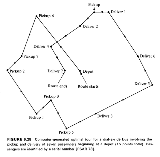
By using our theorem we can conclude that, for large n, the expected
length of the bus route is bounded from below and above by  Kn and
2K, respectively (K 0.765).
For the lower bound, we ignored the
destination-after-origin restriction, while for the upper bound we assumed
that the bus visits all origins first and then alI delivery points. We have
also ignored any restrictions that may be related to bus capacity. The fact
that the route is not a tour but an open path is not important since, in the
limit as n becomes large, the length of the last leg (from the final delivery
point to the origin of the bus) is insignificant by comparison to the length
of the rest of the tour. Sharper bounds and more realistic cases for
dial-a-ride systems are discussed by Stein who has developed several limit
theorems for this problem [STEI 78].
Kn and
2K, respectively (K 0.765).
For the lower bound, we ignored the
destination-after-origin restriction, while for the upper bound we assumed
that the bus visits all origins first and then alI delivery points. We have
also ignored any restrictions that may be related to bus capacity. The fact
that the route is not a tour but an open path is not important since, in the
limit as n becomes large, the length of the last leg (from the final delivery
point to the origin of the bus) is insignificant by comparison to the length
of the rest of the tour. Sharper bounds and more realistic cases for
dial-a-ride systems are discussed by Stein who has developed several limit
theorems for this problem [STEI 78].
In closing this section, we note that, as long as points are reasonably
well "spread around" over a region, the expression 0.765
often provides
good approximations to the length of optimum TSP tours, even in cases when
the n points are not quite independently located or when the probability
distribution for the location of individual points is not exactly uniform
over the region. For instance, it has been estimated that the optimum tour
through 48 major cities, one in each of the 48 continental states in the
United States, and Washington, D.C., is 10,070 miles long, assuming Euclidean
metric [BEAR 59]. Using instead the formula 0.765  with A the area of
the continental United States (= 3,022,400 square miles), one obtains 9,310
miles, for an error of only about -7.5 percent, despite the fact that the 49
cities are far from randomly distributed, since most of them are located at
the outer boundaries of the region (Atlantic and Pacific coasts, Great Lakes
region), with a further disproportionate concentration of almost one third
of the cities in a small part of the country (Northeast).
with A the area of
the continental United States (= 3,022,400 square miles), one obtains 9,310
miles, for an error of only about -7.5 percent, despite the fact that the 49
cities are far from randomly distributed, since most of them are located at
the outer boundaries of the region (Atlantic and Pacific coasts, Great Lakes
region), with a further disproportionate concentration of almost one third
of the cities in a small part of the country (Northeast).
R. Karp has written an excellent paper that shows how, through judicious
partitioning of the area in which the points lie, good TSP tours can be
constructed in problems that may involve thousands of points by taking
maximum advantage of the limit theorem of this section [KARP 77].
|


