Unit 4 : Graphing

Those with graphing calculators or access to plotting programs may think that this unit is unnecessary. There are several schools of thought on this subject, and for current purposes, this unit is included for completeness. One should not have to resort to mechanical aids to make rough sketches of simple functions. Additionally, the properties of curves, interpreted from the derivatives of the functions that the curves represent, is an important part of knowing calculus.

For a specific example of using a program (Maple) for graphing of functions, see Plotting Functions of a Single Variable on MAPLE, Xdvi or PDF; these notes were written in conjuction with a self-paced class in Differential Equations, and involve functions that are far from simple. However, the commands may be adapted for other functions.

Curve sketching uses the first and second derivatives to locate points of interest on the curve. To sketch the curve of y=f(x), we first find where the function reaches maxima and minima. Other than places where the curve is not "smooth" (i.e., |x| is not smooth at x=0), a maximum or minimum occurs only when the first derivative is zero. (One way to see this: for a maximum, the curve must stop going up and start going down. Thus either it passes through a point where it is level, and thus y´=0, or the derivative is not continuous, which is another way of saying the curve isn't smooth.) To aid the accuracy of our sketch, we also obtain information from the second derivative. This informs us of the rate at which the slope of the curve is changing. If this rate is positive, the slope is becoming steadily larger. Geometrically, the curve is concave up or ``holding water.'' Similarly, if y´´<0 the curve is concave down. Solving for the points where the second derivative is zero gives us the places where concavity might change.

A few cautions about curve sketching: Just because a derivative is zero at a point doesn't necessarily mean that the derivative changes sign in the vicinity of that point; it could go from positive to zero and back to positive. (An example is y=x³ in the vicinity of the origin.) Also, remember which function y, y´, or y´´ you want to use at the moment. If, for example, y´´=0 at x=5, graph the point by finding the values of y and y´ at x=5, and draw the curve through that point as a striaight line with that slope. Finally, be careful of discontinuities in the function or its derivatives. Position, slope and concavity can all change drastically at a discontinuity.

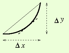
A second topic that will be covered here that doesn't quite fit anywhere else is the Mean Value Theorem and a useful application of it - L'Hôpital's Rule.

First, the Mean Value Theorem. The primary reason to care about this theorem is that it is used to prove many other results we care about even more. For the Mean Value Theorem, we assume a section of a smooth curve (the first derivative is continuous). A sketch of such a curve is shown:

We will let

where the differences (``Delta - x'' and ``Delta - y'') are the changes in the respective coordinates as the curve is traced from one endpoint of the section to the curve to the other.The Mean Value Theorem states that

for some point on the curve section. Finding such a point is rarely of any interest; we simply need to know that such a point exists in future proofs. Look at pictures in the text; the Mean Value Theorem is quite intuitive.

Aside: For a parabolic arc, the point where the slope is equal to the ratio c is at the midpoint of the x - range.

Now that we have the Mean Value Theorem, we can, as promised, prove something interesting: L'Hôpital's Rule. You remember from elementary school that 0/0 lacks meaning. If, instead, we have two functions f(x) and g(x) which both approach zero at x₀, sometimes the limit

does have a value. As a simple example, consider f(x)=x² and g(x)=x as x approaches zero. In this case, the ratio f(x)/g(x) is x if x is not zero, and the limit as x approaches 0 is 0. L'Hôpital's rule gives us a way to evaluate more general cases which cannot be factored so simply:

If this limit is still 0/0 then take derivatives again.

Remember that c/0, for all values of c other than zero, ``is'' infinity. To say this as properly as we can for our purposes,

Similarly, we can and will say that

L'Hôpital's Rule is also valid for another ``indeterminant form'';

can often be masagmed into one of the previous two forms by suitable algebra. As as simple example,

As a not-so-simple example,

The proof of L'Hôpital's Rule is not overly difficult; it is virtually a corollary of the Mean Value Theorem. One final note on indeterminant forms: common sense often finds an answer before repeated applications of L'Hôpital's Rule; look for simple transformations, such as dividing numerator and denominator by xⁿ, that will speed the job.

Objectives:

Upon completion of this unit you should be able to

Sketch curves and indicate regions of positive slope, negative slope, positive and negative concavity.
Understand the Mean Value Theorem.
Apply L'Ho&pcirc;ital's Rule to appropriate limits.

Suggested Procedure:

Read Simmons 4.1-4.2 and 12.1-12.3
Sorry, there are not yet any World Web Math entries on this topic.
Again, you need to work lots of problems, especially to get the hang of graphing. Simmons has problems on pp. 91, 94. The problems vary widely in difficulty. Work your way up to the harder ones by solving many of the easier ones. For L'Hopital's rule, do problems from sections 12.2 and 12.3.
Take a Sample Unit Test, Xdvi or PDF.
Ask your instructor to give you a unit test.

Independent Study page | Calculus page World Web Math Categories Page

watko@mit.edu

Last modified July 31, 1998