 Unit 5: More Applications of Differentiation
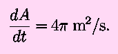
The next application of the derivative is related
rates. The usual
problem here is to have a function, say the area of a circle of radius
r,
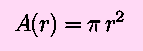 and a derivative, such as dr/dt=4 m/s, and we wish to find
another derivative, in this case dA/dt. In other words, to
relate the unknown rate to the known rate. There are two
basic methods, which are roughly equivalent:
and a derivative, such as dr/dt=4 m/s, and we wish to find
another derivative, in this case dA/dt. In other words, to
relate the unknown rate to the known rate. There are two
basic methods, which are roughly equivalent:
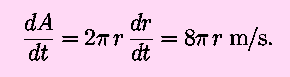
- Use implicit differentiation. In this case, differentiate with
respect to time:
- Use the chain rule:
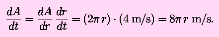
Note that in both cases we need to know the current value of the
radius to specify the change in the area. When r=0.5 m,
 Note that these problems can get tricky, either because of a large
number of derivatives floating about, or because of difficulty in
setting up the geometry of the situation. Also note that in this
case, the units of the answer are what they should be.
Note that these problems can get tricky, either because of a large
number of derivatives floating about, or because of difficulty in
setting up the geometry of the situation. Also note that in this
case, the units of the answer are what they should be.
Next, we have max-min problems. The basic situation
here is that we have several quantities related to each other by
various formulae. We wish to either minimize or maximize one of the
quantities by appropriate choices for the values of the others. Recall
that, in a smooth region, the maxima and minima occur when the first
derivative is zero. So our method is to set up a derivative, set the
expression for the derivative equal to zero and solve, and then
``solve backwards'' to get the desired values. A typical example is
the case of a farmer who lives next to a straight stream. He has
bought 100 m of fence and wishes to enclose as much pasture as
possible, using the stream as one side of the pasture. He also insists
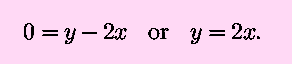
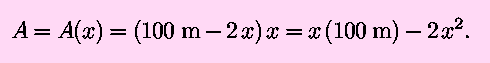
that the pasture be rectangular. To set this up, we call the length of
the side opposite (or parallel to) the stream y, the common
length of each one of the sides adjacent to the river x,
the area A and obtain
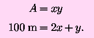 At this point, we could choose either x or y to
be the variable for which we solve. For consistency with previous
usage, we will solve for y as a function of x.
At this point, we could choose either x or y to
be the variable for which we solve. For consistency with previous
usage, we will solve for y as a function of x.
We could eliminate either variable in favor of the other; that will
be done later, as a check. Using implicit differentiation,
differentiate the first of the above equations with respect to
x to obtain
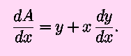 Differentiate the second equation to obtain
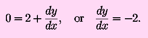 Setting dA/dx=0 and subsituting dy/dx=-2,
 Subsituting into the second of the first set of equations (sometimes
known as ``Solving backwards'') gives x=25 m,
y=50 m, and A=1250 m².
Subsituting into the second of the first set of equations (sometimes
known as ``Solving backwards'') gives x=25 m,
y=50 m, and A=1250 m².
How do we know this is the maximum, and not a minimum? Well, it's
fairly obvious in a simple example like this, but in general:
- Check near the supposed maximum; x=24 m,
y=52 m gives A=1248 m² and
x=26 m, y=58 m gives
A=1248 m². Both are smaller than the solution, so
we're okay. (By the way, it is not a coincidence that changing the
value of x by the same amount either way gives the same
area.)
- Check borderline cases or discontinuities. Here, x=0,
y=100 m and x=50 m,
y=0 both give A=0.
- Use common sense. Don't let lengths, areas or volumes go
negative. We found only one extreme, and that can't be a minimum, as
that would mean there is no maximum.
The trick to max-min problems is setting things up so that when you
solve for the derivative equal to zero, you actually have an
equation you are capable of solving.
To check, as promised, substitute
y=100 m-2x into the original expression for
the area to obtain
 Differentiating with respect to x and setting the
derivative equal to zero gives
Differentiating with respect to x and setting the
derivative equal to zero gives
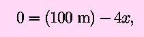 which is readily solved for x=25 m, as before.
As another use of differentiation for this unit, we present
Newton's method for approximating roots of equations.
This section is completely optional. The idea is as
follows: we have an equation f(x)=0, and wish to
solve for a value of x. We start with a guess,
x0, and try to improve the guess. At the point
(x0, f(x0)),
the tangent to the curve is given by the equation
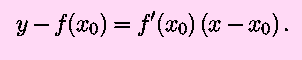 We solve this to find the point where the tangent line crosses the
x-axis, where y=0. Denoting this value of
x as x0,
We solve this to find the point where the tangent line crosses the
x-axis, where y=0. Denoting this value of
x as x0,
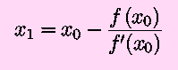 x1 = x0 - (f(x0) /
f'(0))
The above procedure is indicated by considering a figure of the curve
of a typical function:
x1 = x0 - (f(x0) /
f'(0))
The above procedure is indicated by considering a figure of the curve
of a typical function:
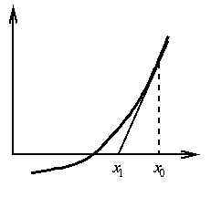 If we started somewhere near the desired root, and
f(x) is well-behaved (we'll leave
``well-behaved'' ill-defined for the moment), then
x1 will be closer to the root than
x0. We continue the process, calculating
x2, x3, etc., until we are
near enough to the root to be satisfied. (``Near enough'' is commonly
defined in terms of the number of digits of accuracy possessed by the
calculator or computer in use, or given in a particular problem at
hand.)
If we started somewhere near the desired root, and
f(x) is well-behaved (we'll leave
``well-behaved'' ill-defined for the moment), then
x1 will be closer to the root than
x0. We continue the process, calculating
x2, x3, etc., until we are
near enough to the root to be satisfied. (``Near enough'' is commonly
defined in terms of the number of digits of accuracy possessed by the
calculator or computer in use, or given in a particular problem at
hand.)
For an example that is easily checked, consider
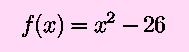 which leads to, with an extension of the notation,
 that is, we wish to find the square root of 26. Of course, any
calculator that could perform the calculations necessary to use
Newton's Method will be able to find the square root immediately.
This is for demonstration purposes only.
that is, we wish to find the square root of 26. Of course, any
calculator that could perform the calculations necessary to use
Newton's Method will be able to find the square root immediately.
This is for demonstration purposes only.
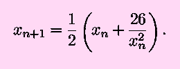
Starting with x0=5 gives
x1=5.1 (this first step might even be done
without a calculator). Then, x2=5.00990196. To
this same precision, the square root of 26 is 5.00990195. Note that
this took only two iterations.
When Newton's method works, it works fairly well. For finding things
like roots to quadratics and cubics, the number of correct digits in
the answer roughly doubles at each step. For finding roots of
functions more complicated than polynomials, Newton's method is less
reliable. The text shows examples where Newton's method fails
entirely.
Objectives:
You should understand what the Mean Value Theorem says; don't worry
excessively about its proof. You should be able to find values for
indeterminant forms, using L'Hopital's Rule where appropriate.
Suggested Procedure:
- Simmons 4.6, 12.1-12.3.
- Sorry, there are not yet any World Web math pages on this topic.
- Do some problems in Simmons
- page 337, several of 1-22 (avoid any containing e or
ln for now).
- Simmons, page 115, 1-5, 9.
- Take the Practice Unit
Test, Xdvi or PDF.
- Ask your instructor for a unit test.
Independent Study page |
Calculus page
World Web Math Categories Page
watko@mit.edu
Last modified August 1, 1998