XCrySDen can display the
crystal (or molecular) structures from the
PWscf input and output files
(here the
pw.x code is meant).
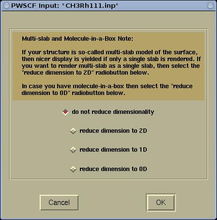
Before visualizing the structure, the program will
query for possible reduction of the structure's
dimension (here periodic dimensions are meant). For
example, molecule has zero periodic dimensions, while
surface (slab) has two periodic dimensions, therefore
it is recommended to display them with the
appropriate number of periodic dimensions.
Here is the periodic query window:
The crystal (or molecular) structure from the
pw.x input file can be displayed either by the
appropriate command line option or from the menu.
From command-line:
- either: xcrysden --pwi file
- or: xcrysden --pw_inp file
Frome menu: select the menu item
File-->Open PWscf
...-->Open PWSCF Input File
The crystal (or molecular) structure from the
pw.x input file can be displayed either by the
appropriate command line option or from the menu.
From command-line:
- either: xcrysden --pwo file
- or: xcrysden --pw_out file
Frome menu: select the menu item
File-->Open PWscf
...-->Open PWSCF Output File
There are four types of coordinate extraction modes,
and this will be queried with the following window:
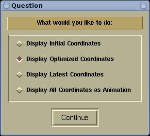
Below is the description of the four types of
extraction modes.
The
Display Initial Coordinates mode will
display the initial coordinates printed at the
beginning of the
pw.x output file, i.e., those
printed in the following manner:
     site n.     atom                  positions (a_0 units)
         1           H   tau(  1) = (  -.1657590  -.0955104  1.2559945  )
         2           H   tau(  2) = (   .1659009  -.0954643  1.2557377  )
         3           H   tau(  3) = (   .0000000   .1917322  1.2548077  )
         4           C   tau(  4) = (   .0000000   .0000000  1.1886906  )
         5           Rh  tau(  5) = (   .0000000   .0000000   .8054534  )
         6           Rh  tau(  6) = (   .7499998  -.4330126   .8054534  )
         7           Rh  tau(  7) = (   .4999998   .0000000   .8054534  )
         8           Rh  tau(  8) = (   .2499999  -.4330126   .8054534  )
         9           Rh  tau(  9) = (  -.2499999   .1443376   .4082482  )
        10           Rh  tau( 10) = (   .0000000  -.2886750   .4082482  )
        11           Rh  tau( 11) = (   .4999998  -.2886750   .4082482  )
        12           Rh  tau( 12) = (   .2499999   .1443376   .4082482  )
        13           Rh  tau( 13) = (  -.4999998   .2886750   .0000000  )
        14           Rh  tau( 14) = (  -.2499999  -.1443376   .0000000  )
        15           Rh  tau( 15) = (   .2499999  -.1443376   .0000000  )
        16           Rh  tau( 16) = (   .0000000   .2886750   .0000000  )
The
Display Optimized Coordinates mode will
display the optimized coordinates, therefore this mode
is useful only for the output file of geometry
optimizations. If the optimized coordinates are not
found in the output file, the program will signal an
error. The optimized coordinates are printed in the
following manner in the output file:
     End of BFGS geometry calculation

     Final energy            =   -1226.4092020951 ryd

     Saving the approximate inverse hessian


CELL_PARAMETERS (alat)
   1.000000000   0.000000000   0.000000000
   0.000000000   1.414213562   0.000000000
   0.000000000   0.000000000   3.150000000

ATOMIC_POSITIONS (alat)
O       -0.000066379  -0.513244840   1.345933583
N        0.000016050  -0.730745427   1.464247866
N       -0.000018075  -0.898866014   1.326587159
Pd      -0.000083375  -0.711492446   1.013218636
Pd       0.499979720  -0.706754811   0.987470168
Pd       0.000094941   0.000039404   0.983520698
Pd       0.500073136   0.000254615   0.980957462
Pd      -0.248933604  -0.357455663   0.757427630
Pd       0.248979012  -0.357447626   0.757410448
Pd      -0.248500404   0.358259400   0.758511634
Pd       0.248539175   0.358243548   0.758490039
Pd       0.000000000  -0.707106780   0.500000000
Pd       0.500000000  -0.707106780   0.500000000
Pd       0.000000000   0.000000000   0.500000000
Pd       0.500000000   0.000000000   0.500000000
Pd      -0.250000000  -0.353553390   0.250000000
Pd       0.250000000  -0.353553390   0.250000000
Pd      -0.250000000   0.353553390   0.250000000
Pd       0.250000000   0.353553390   0.250000000
Pd       0.000000000  -0.707106780   0.000000000
Pd       0.500000000  -0.707106780   0.000000000
Pd       0.000000000   0.000000000   0.000000000
Pd       0.500000000   0.000000000   0.000000000
The
Display Latest Coordinates mode will
display the latest coordinates in the output file. If
the latest printed coordinates are the optimized
coordinates, then these will be displayed.
The
Display All Coordinates as Animation
mode will display the all the coordinates found in the
output file, including the initial coordinates. This
mode is useful for geometry optimizations and molecular
dynamics calculations. The user will have the
possibility to animate forth and back through all the
"images" of the involving structure during the
calculation.
Whenever a given crystal structure is displayed by
XCrySDen, it
is possible to graphically select a k-path for the band
structure calculation (
spaghetti plot) via the
Tools-->k-path
Selection menu.
Read here the description of how to
select graphically the k-path.
IMPORTANT: to save the selected k-path in the
format compatible with the PWscf, make sure to save
the file with the .pwscf extension (example:
my_kpath.pwscf).
To visualize charge densities, STM images, and
similar properties with
XCrySDen user needs to
calculate this property and store the data into the
XSF
format. Here is the sequence of the PWscf tasks that
needs to be performed:
- the SCF calculation: pw.x < pw_input >
pw_output
- the post-processing calculation, where a given
property is selected: pp.x < pp_input >
pp_output
- calculated property needs to be converted to the
XSF format
using the chdens.x program: chdens.x
< input > output


![[Figure]](img/xcrysden-picture-small-new.jpg)