Probabilistic Latent Component Analysis

This work has been primarily based off two papers by Paris Smaragdis, “Shift-Invariant Probabilistic Latent Component Analysis” (Smaragdis & Raj 2007) and “Separation by “humming”: User-guided sound extraction from monophonic mixtures” (Smaragdis & Mysore 2009). Please visit his web-page and give them a read if you want to know more. They are good reads.

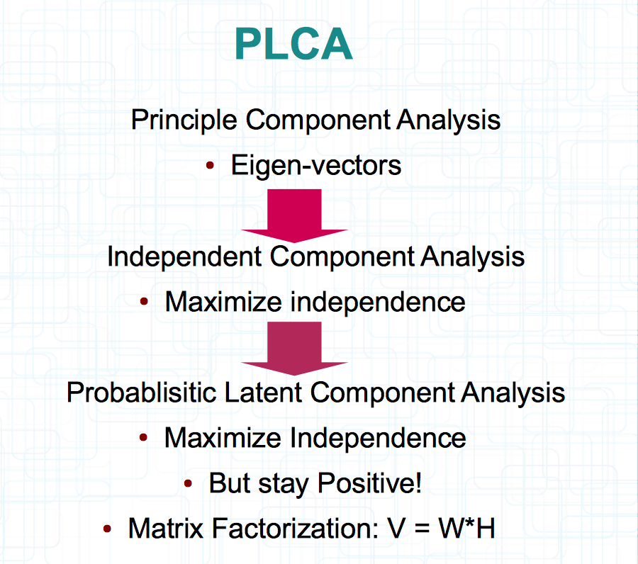Some of the earliest work in audio separation and extraction was done using Principle Component Analysis, maximizing component variance. Subsequently, Independent Component Analysis, targeting components of maximal independence became dominant for finding latent components. But ICA decomposition yields results that are statistically but not necessarily interpretable. For instance, ICA will find components with negative vectors. With the example of audio, there are no negative frequencies so these decompositions are unintuitive.

PLCA is a form of Non-Negative Matrix Factorization that looks to maximize independence similarly to ICA, but forces the results to be positive yielding understandable results. PLCA is an Expectation-Maximization algorithm that models a mixture of independent distributions. Each distribution is considered an independent component, z, latent within the data. The idea is to discover what these latent components and where are they.

Here’s a more complex but easily understandable example provided from Smaragdis’s work:

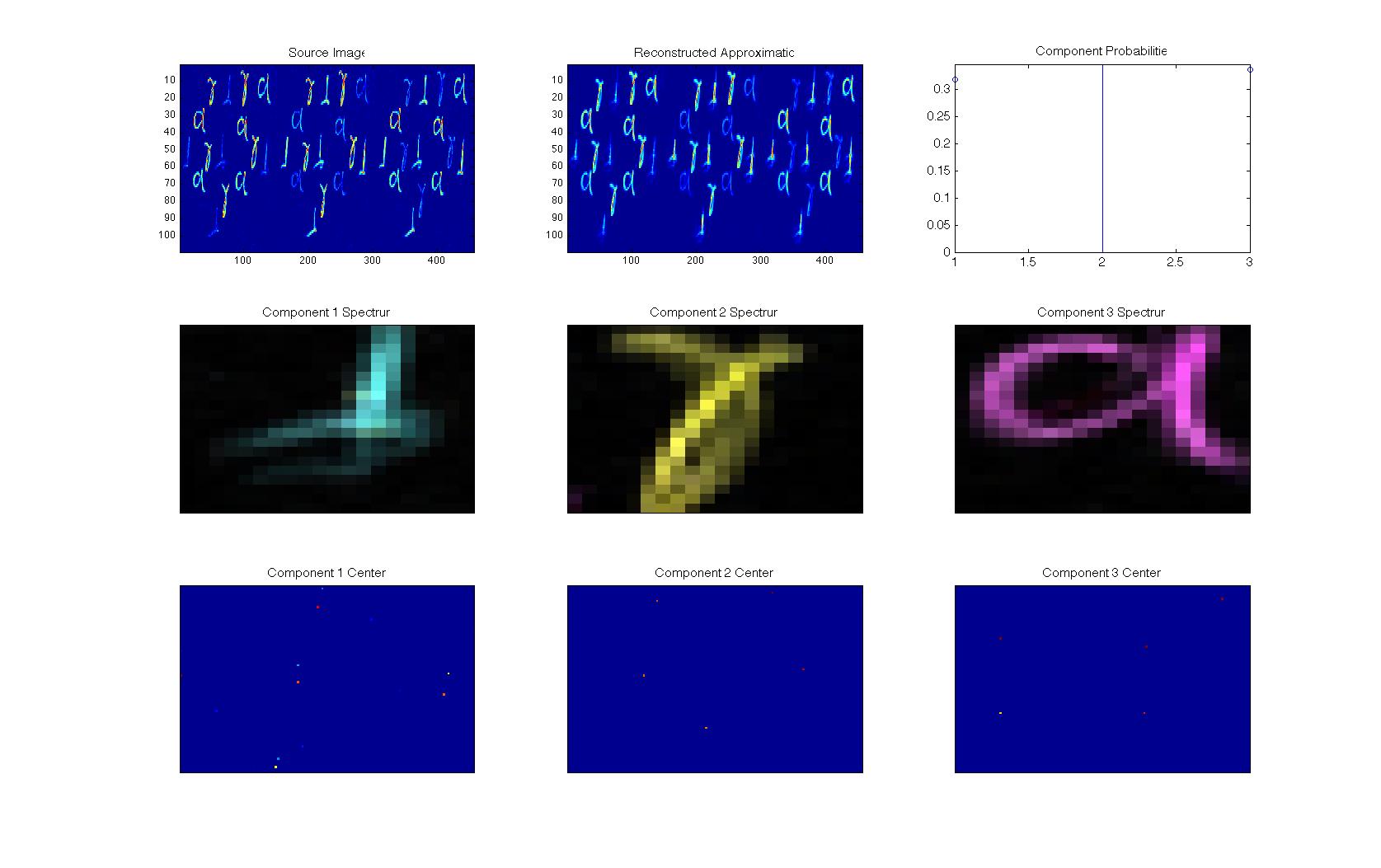
Looking at the initial image, it is possible to see that there are three main shapes. These are identified as components with 3 main properties. The mixture distributions itself shown in the second row. The bottom row displays the discovered centers of these mixtures while the third image in the top row relates the probability of each of these three components occuring. Multiplying (or convolving in this case) the three component properties together results in an approximation of the original image. Each component will be an average of the similar originals. The algorithm is standard EM in that in the estimation stage, it calculates the contribution of each component to the sum spectrum and in the maximization the three components property marginals are re-weighted. For the actual detailed math, please refer to the referenced papers.

Audio is a 2-D PLCA example. The first step is to switch to the fourier domain and use the frequency spectrum for decomposition. Here the component z is the spectral content of a specific note event or sound. It is decomposed into three properties: the spectral signature p(f|z), the magnitude over time p(t|z) and the component likely hood p(z). This is demonstrated below:

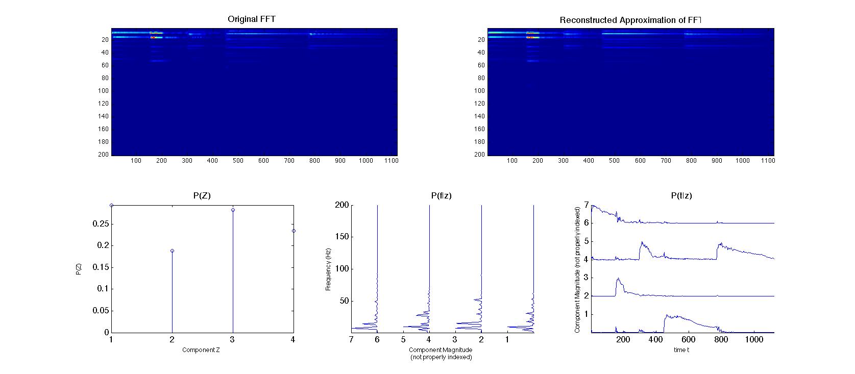
The example used in this case is a five event, four note pattern on the piano. The three graphs can be easily understood to depict the frequency spectrum generated by each note, the times at which those notes sound, and the overall probability of each.

One of the unknowns in the algorithm is how many components or notes a sample has. In both these examples, we've known and can specify appropriately. A slightly different version of the above is run requesting five components. This time the algorithm is run to find 5 components:

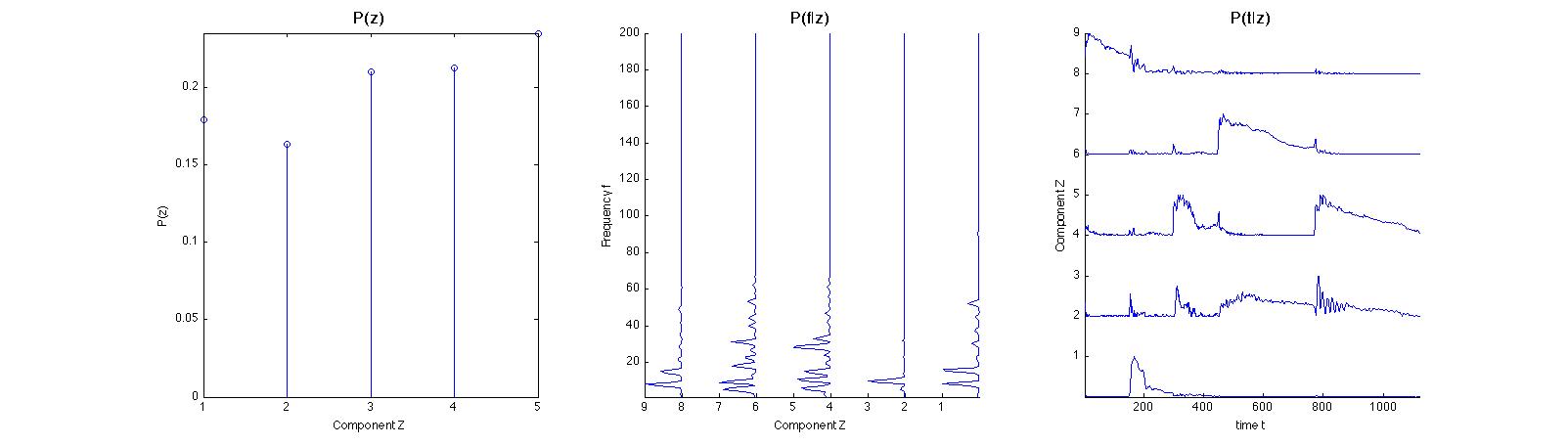
It is relatively easy to discern that the 2^nd component is an conglomeration of the other 4 components and not actually very informational. In separation, this is mildly problematic but discoverable. In extraction it introduces more possibility for error.

Next- Extraction Using PLCA & Mimicry