Results- It Works!

Full reports on each data set will be linked shortly. But for now, here are results for the extraction of the primary vocal line from Oasis's Wonderwall. It was extracted using a mimic where I sang the lines after a couple rehearsals (and learning how to avoid too much sibilant hitting the microphone.

The extraction posted was done with M = 9 target components and N = 150 backing components using 30 iterations. It does not include the Bayes Mask yet.

And now for some stats on the voice extraction from Oasis's Wonderwall using a sung mimic.

Stats & Discussions:

The axis for all MSE graphs except the first two been inverted so that high always means better. This makes for better consistency between graphs.

Naïve Bayes

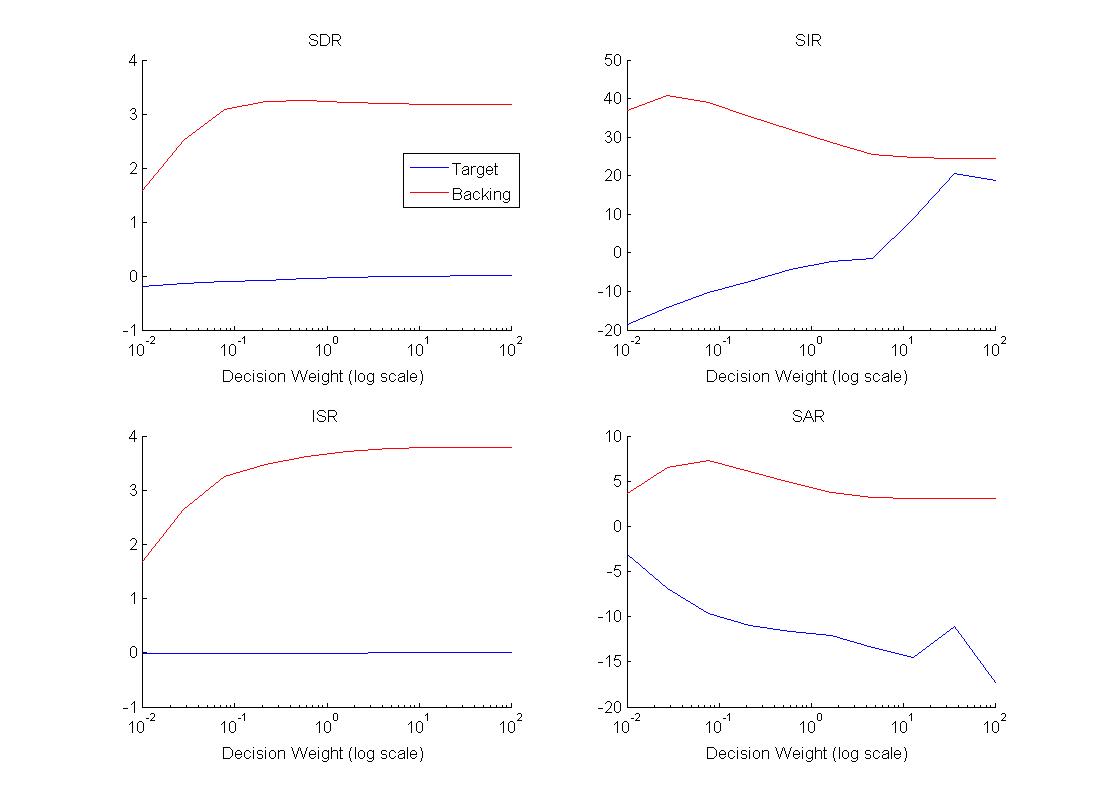
This is for comparison. This is a test run extracting the vocals using the mimic to inform basic Bayes Classification on each spectrum/time element with different risk. I've included the results when running it with equal cost for making an error or getting it right. The odd thing here is that it still dominantly retains the sound of the mimic even though the mask is applied on the mix to get the final audio. Changing the weight to favor more of the original in the result does improve the sound. But the biggest problem with this approach is the significant amount of artifact from phase (SAR). It simply doesn't sound good.

Wonderwall segment after naive Bayes Classification

BSS Tests in extraction using Bayes Classifiers

Algorithm Iterations

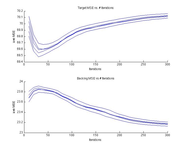
An exception to the inversion of MSE graphs is here where the MSE is tracked over multiple iterations of the PLCA algorithm. Oddly, for the target, somewhere around 30 is the optimal iteration length in this case.

Predictor for M?

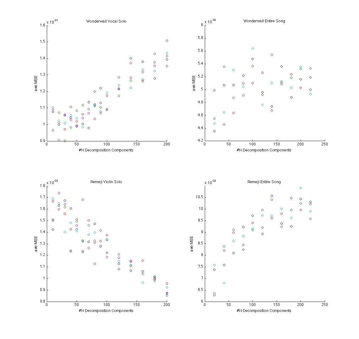
It was originally hoped that the correct choice of M would be easily disceranable from a run looking at MSE on the target audio compared to it's approximation. Although this had promise in some cases, trends do not seem to necessarily be relevant between different songs. For instance in the graph (lower is better) it suggests M should be less than 60 for the Wonderwall vocal. Used on a violin sample, the more components the better. It is actually known (see below) that M for Wonderwall should be closer to 9, not discernable here. Hence, MSE of the target versus it's approximation was deemed not very helpful.

Selection of M & N

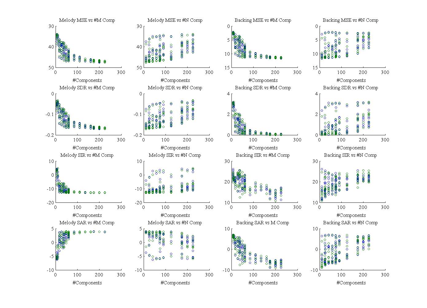
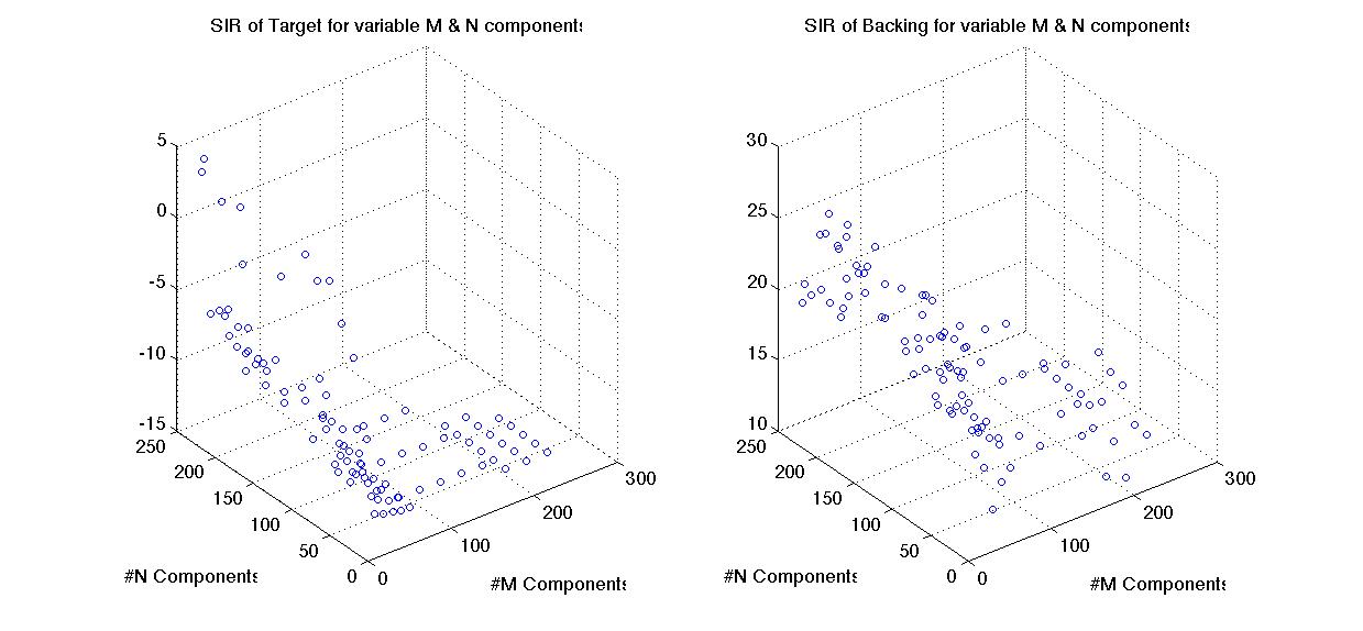
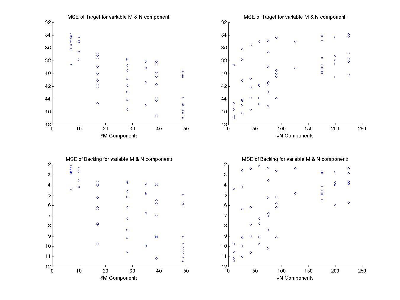
Here's a look of M compared to N. Clearly, lower M is better for the extraction which is expected as there are only three actual notes in the vocal melody here. However choosing M = 3 turned out to be too limiting. It reproduced a good pitch extraction but lost the words. Raising M to 9 restored most of the words. Increasing it further will decrease the amount of the target that is lost but at the cost of increasing backing leaking in. Notice also that there is a bit of an inverse relationship between preferred N vs. M. A lower N paired with high M will lead to a better backing extraction.

Wonderwall extraction using M = 3

If you prefer a 3D depiction of the above, here is an example. Personally I find it more confusing:

Now it is clear smaller M is preferable, taking a reduced view provides an easier chance to see where the best M might lie. In this case I am presenting the reduction for MSE even though SIR is preferable for achieving optimality. As mentioned MSE is less costly to compute and it is visible in this graph that there is a clear drop in MSE from its maximum between 10 & 17 components. This mimics the SIR results although less dramaically. This most likely matches with where M is over described. Looking for this drop in MSE should help discover optimal M for future cases.

Sparsity

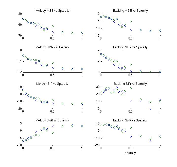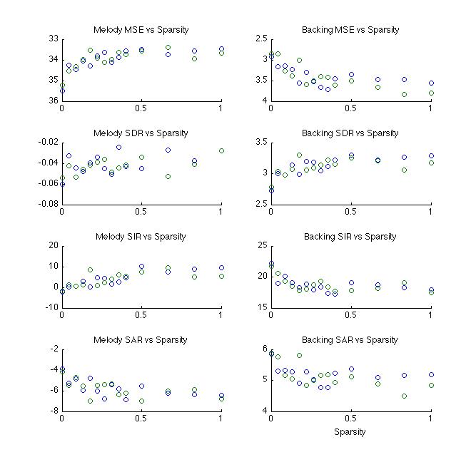
Sparsity test were run with 30 iterations and M continuing to equal 9. Adding sparsity in Z essentially works to filter out weaker components. It would be expected that this would reduce information. Components that may end up with significance in the wrong class set would hopefully be weaker and their removal would improve audio. It is expected that it would be result in poorer statistical results, but it turns out it does not sound very good either. Too much information is apparently removed.

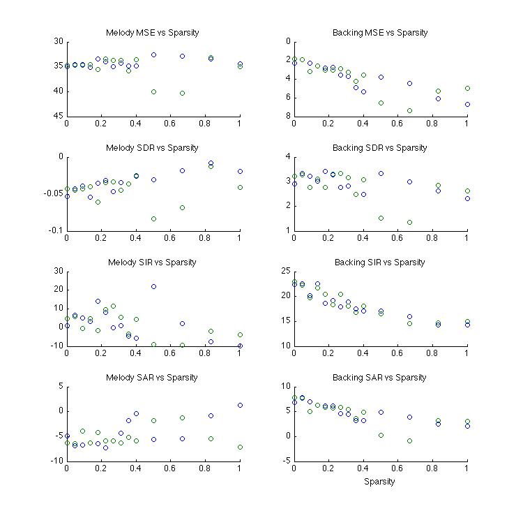
Sparsity in W and H would be expected to clean-up frequency and timing respectively. For instance, audio that leaks into the lead when it is not playing might hopefully be reduced by changes to H. Generally this held true to produce positive results although it did significantly increase artifact. For the resulting audio it is questionable if it actually sounds better or not when sparsity in both these measures are used beyond small quantities. These results apply to sparsity applied jointly on W & H. Sparsity in W, H, & Z seemed to produce unpredictable results. The example included here is surprisingly good in that the result is really almost exclusively voice. There is also significant artifact and personally, the sound is far too pale.

The audio examples are three cases where the addition of sparsity improves the SIR. They are taken from the audio linked to the highest SIR achieved.

Example Audio: Best SIR from Sparsity introduced in W

Example Audio: Best SIR from Sparsity introduced in W & H

Example Audio: Best SIR from Sparsity introduced in W, H, & Z

Below: Sparsity applied to W. Above right: Sparsity appled to Z

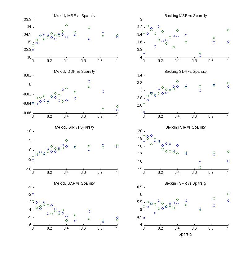
Below: Sparsity applied to H

Below: Sparsity applied to W & H

Below : Sparsity in W, H, & Z

Bayes Decision Classification:

Bayes Binary Masking after PLCA works well to further clean up the audio. The plot below suggests that some masking is preferable than none. Experience has shown that the optimal ratio is also not static. Again, what is optimal for melody, is often opposed to optimality for backing. Worth remembering too is that this does introduce additional artifact but closer to even cost, it is within reason.

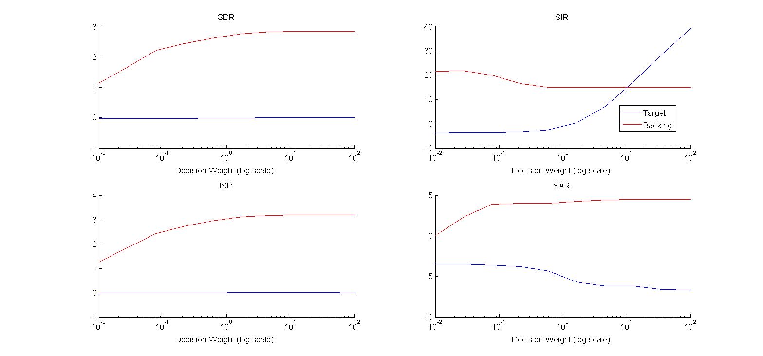
Impact of using Bayes Decision Classification with differing Risk

Example Audio: Extraction with Bayes Decision Mask applied with cost ratio 0.8

Next: Conclusions & The Future