Let's denote the time at the nth time-step by tn and the
computed solution at the nth time-step by yn, i.e.,
![]() .
The step size
h (assumed to be constant for the sake of simplicity) is then given by
h = tn - tn-1.
Given
(tn, yn), the forward Euler method (FE) computes yn+1 as
.
The step size
h (assumed to be constant for the sake of simplicity) is then given by
h = tn - tn-1.
Given
(tn, yn), the forward Euler method (FE) computes yn+1 as
| (6) |
The forward Euler method is based on a truncated Taylor series expansion, i.e., if we expand
y in the neighborhood of t=tn, we get
| (7) |
A convergent numerical method is the one where the numerically computed solution approaches the exact solution as the step size approaches 0. Once again, if the true solution is not known a priori, we can choose, depending on the precision required, the solution obtained with a sufficiently small time step as the 'exact' solution to study the convergence characteristics.
Another important observation regarding the forward Euler method is that it is an explicit
method, i.e., yn+1 is given explicitly in terms of known quantities such as yn and
f(yn,tn). Explicit methods are very easy to implement, however, the drawback arises from
the limitations on the time step size to ensure numerical stability.
In order to see this better, let's examine a linear
IVP, given by
dy/dt = -ay, y(0)=1 with a>0. As we know, the exact solution
![]() ,
which is a stable and a very smooth solution with
ye(0) = 1 and
,
which is a stable and a very smooth solution with
ye(0) = 1 and
![]() .
Now, what is the
discrete equation obtained by applying the forward Euler method to this IVP? Using Eq. 7, we get
.
Now, what is the
discrete equation obtained by applying the forward Euler method to this IVP? Using Eq. 7, we get
| yn+1 = yn -ah yn = (1-ah) yn = (1-ah)2 yn-1 = ... = (1-ah)n y1 = (1-ah)n+1 y0. | (8) |
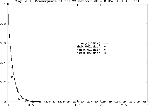
These results can be better perceived from Figures 1 and 2. The test problem is the IVP given by
dy/dt = -10y, y(0)=1 with the exact solution
![]() .
The stability criterion for the
forward Euler method requires the step size h to be less than 0.2. In Figure 1, we have shown
the computed solution for h=0.001, 0.01 and 0.05 along with the exact solution1.
As seen from there, the method is numerically stable for these values of h and becomes more accurate as h decreases.
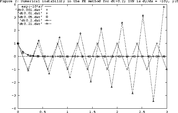
However, based on the stability analysis given above, the forward Euler method is stable only
for h < 0.2 for our test problem. The numerical instability which occurs for
.
The stability criterion for the
forward Euler method requires the step size h to be less than 0.2. In Figure 1, we have shown
the computed solution for h=0.001, 0.01 and 0.05 along with the exact solution1.
As seen from there, the method is numerically stable for these values of h and becomes more accurate as h decreases.
However, based on the stability analysis given above, the forward Euler method is stable only
for h < 0.2 for our test problem. The numerical instability which occurs for
![]() is shown in Figure 2. For h =0.2, the instability is oscillatory between
is shown in Figure 2. For h =0.2, the instability is oscillatory between ![]() ,
whereas for h>0.2, the amplitude of the oscillation grows in time without bound, leading to an
explosive numerical instability.
,
whereas for h>0.2, the amplitude of the oscillation grows in time without bound, leading to an
explosive numerical instability.
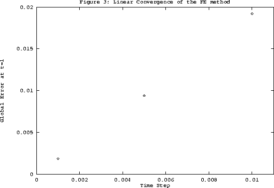
The convergence of the solution can be analyzed quantitatively. Let's look at the
global error
gn = |ye(tn) - y(tn)| for our test problem at t=1. We know that
the local truncation error (LTE) at any given step for the Euler method scales
with h2. Hence, the global error gn is expected to scale with nh2. However,
for the integration within a fixed time interval, n is proportional to 1/h.
So the global error gn at the nth Euler step is proportional to h. This
result is confirmed by the computational results presented in Figure 3, where
the global error at t=1 is plotted against the time step size h.
The conditional stability, i.e., the existence of a critical time step size
beyond which numerical instabilities manifest,
is typical of explicit methods such as the
forward Euler technique. Implicit methods can be used to replace explicit ones
in cases where the stability requirements of the latter impose stringent conditions on the
time step size. However, implicit methods are more expensive to be implemented for non-linear
problems since yn+1 is given only in terms of an implicit equation. The implicit analogue of
the explicit FE method is the backward Euler (BE) method. This is based on the following Taylor
series expansion
| (9) |
| (10) |
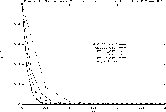
Well, why do we resort to implicit methods despite their high computational cost? The reason is
that implicit techniques are stable. Let's examine this for the same linear test problem
we considered in the context of the FE method:
dy/dt = -10 y, y(0) = 1. In the case of
linear problems, using BE is as easy as using FE, applying Eq. 11, we have
| (11) |