Massachusetts Institute of Technology
Department of Urban Studies and Planning
|
11.188: Urban Planning and Social
Science Lab |
Lab Exercise 4: Vector Spatial Analysis
Out: March 15, 2021; Due: Wednesday, March 24, 2021, via Stellar
Overview
In this exercise you will use a few of the spatial analysis capabilities of QGIS to:
- Examine the location patterns of Cambridge stores by using the 'spatial join' tools to tag store location data (convenience stores, coffee shops, and pet stores) with the demographic characteristics of their neighborhood. (This is a 'point-in-polygon' operation.)
- Create an 800 meter buffer around Ames St.
- Estimate the number of children living near Ames Street by:
- Overlaying the Ames St. buffer with the Cambridge blockgroup data.
- Apportioning young children in each blockgroup that is split by the buffer, in proportion to the block group area that falls within the buffer.
- The in-lab discussion notes are here: Lab #4 notes
Preliminaries
Copy all parts of the following shapefiles from the class data locker in the directory \\afs\athena.mit.edu\11.188\data to C:\TEMP\lab4 or some other local drive. Alternatively, these shapefiles are bundled, with a few additional files and tables, into a zipfile available on Stellar as 11.188_lab4_data.zip:
camb_area_lu_1999.shp
Land use for towns in and around Cambridge in 1999 per MassGIS. In addition, the 'qml' style file, camb_lu21_style-massgis2.qml, provides MassGIS color for the 21 codes in 'lu21_code'.
cambbgrp2010.shp
U.S. Census 2010 block groups for Cambridge. Make sure NOT to use the older 1990 cambbgrp shapefile from earlier exercises
2010_cambtigr.shp
U.S. Census 2010 TIGER file for Cambridge from MassGIS
cambridge_convenience.shp
Convenience stores in Cambridge
cambridge_coffee.shp
Coffee shops in Cambridge
cambridge_pet.shp
Pet stores in Cambridge
R10905063_SL150.xls Spreadsheet with selected ACS 2009-2013 block group census data for Massachusetts 2009_13_ACS_Age_SocialExplorerTable.xls Spreadsheet with ACS data from Social Explorer with Cambridge block groups counts of kids by age group. We obtained the addresses for the features in the cambridge_convenience.shp, cambridge_coffee.shp, and cambridge_pet.shp layers from the ReferenceUSA web site on January 27, 2015. We geocoded these addresses using the free TAMU GeoServices platform. We also geocoded 4 retail locations 'manually' using GoogleMaps to obtain a higher match rate. What is geocoding and how does it work? Well, we'll be exploring address geocoding later in the semester.
You are welcome to use the QGIS project document,11.188_lab4_start.qgz, saved within the Lab#4 data package, 11.188_lab4_data.zip. The QGIS project document includes links to the Stamen basemaps and the MassGIS orthophotos that will be helpful to provide neighborhood context as you work through this lab exercise.
Part
1: Point in Polygon Spatial Join and Cluster Analyses
In this part of the lab, you will examine the demographic characteristics of the block groups in which various coffee shops are located. The point coffee shop data is contained in the shape file called cambridge_coffee.shp.
QGIS can do 'point in polygon' overlay operations using a spatial join. We shall join cambridge_coffee.shp and cambbgrp2010.shp so that block group attributes can be added to the coffee shop table. Previously, we have used 'select by location' to highlight features (such as Cambridge housing sales) that are located with specific regions (such as high-income neighborhoods). But highlighting the features is not enough. We would like to add to each row of the Coffee Shop attribute table the census data associated with the block group that contains the coffee shop.
Spatial
Join
- QGIS provides a 'join by location' tool in the Toolbox. Click 'Prociessing / Toolbox' to open the Toolbox window, and then choose 'Vector / General / Join Attributes by Location' to open that tool. Your screen should look something like the QGIS screenshot below.
- The 'Input Layer' with the neighborhood attributes is cambbgrp2010 and the 'Join Layer' is cambridge_coffee.
- Which geometric operation should we use for the spatial join?
- We want to tag the coffee shop that 'intersects' or falls 'within' a particular block group.
- Which fields do we want to append to the coffee shop attribute table?
- We don't need them all. Just bring across the state-county-tract-blockgroup geographic identifier, geoid
- For the 'Join type' choose, "Create separate features for each located feature. (one-to-many)"
- Do you understand this choice?
- The alternative is, "Take attributes of the first located feature only (one-to-one)
- In our case the Cambridge block group boundaries do not overlap and the coffee shops are points. So the relationship is one-to-one and either option will yield the same result.
- Your 'Join Attributes by Location' window should look something like the one below.
- Leave the remaining default parameters unchanged and click 'Run'.
- A temporary layer called 'Joined Layer' is added to the Layer panel.
- Open the cambbridge_coffee attribute table. It should look something like the screenshot below. Notice that each coffee shop has been taged with a 'Geoid' value in the newly added column and that identifies the census block group that the coffee shop falls within.
QGIS with Toolbox ready to select 'Join Attributes by Location'
Tagging each Coffee Shop with its Cambridge Block Group ID

Coffee Shop Attribute Table after adding Geoid field
The 'joined layer' is only temporary. Export the layer into a shapefile called coffee_bgrp.shp. The new shapefile, coffee_bgrp.shp, will be added to your layer panel. Now that we have tagged each coffee shop with its GEOID, we can join it to any table of 2010 block group Census data. Let's use some data from the 2009-2013 American Community Survey that was introduced in last week's lab. The spreadsheet, R10905063_SL150.xls, contains median household income ACS data in addition to geographic identifiers . It is available in the Census_ACS folder of our data locker and also in 11.188_lab4_data.zip. Can you figure out what field to use for the attribute join with coffee_bggrp.shp? It is *not* the Geo_GEOID field that has the prefix '15000US' added to the state-county-tract-block-group identifier. Instead use the column labeled FIPS/ The fields that you use to join the shapefile and the xls table need not have the same name but they do need to contain the same formulation of a block group identifier (state, county, tract, block group). Add R10905063_SL150.xls as a vector data layer and join it to coffee_bggrp.shp.
The field labeled "ACS13_5yr_B19013001" contains the median household income estimates. We could discover this field using the online ACS website or the lookup tables that we used during Lab#2. Map the values in this column using graduated symbls. Follow the same gemeral instructions as in Lab #2, except that you will use the location of coffee shops instead of housing sales. Turn off the block group layer and turn on the Cambridge roads (in the TIGER file) to help provide context for interpreting the map. To provide additional context for interpreting these locations, create a thematic map of land use using the camb_area_lu_1999.shp layer. A file named camb_lu21_style-massgis2.qml contains XML-tagged style information in the QGIS style file format. You can load the style information from the 'style' button on the 'symbology' tab of 'layer properties'.
- For further information about land use codes, check the MassGIS land use code definitions in the 'datalayers' sections of the MassGIS website.
Take a close look at the pattern of coffee shops. Does anything look interesting? Write your observations as requested in Question 1 of the assignment. Prepare a 'layout' PDF of your map and submit this as the answer for Question 2.
For extra credit, or just for fun, redo the spatial join; this time joining the 2010 block groups to the convenience store and pet store shapefiles (this requires a spatial join for each of the store layers) and display them on the map too. Do the additional store locations help you see a pattern?


Part
2: Buffer Analysis
In this part of the lab, you will analyze the demographics of the neighborhood around MIT's biological research facility on Ames Street. You will build on what you learned in the "Simple Buffering" part of Lab 3 to do a more elaborate analysis. In particular, when the buffer boundary cuts through a block group, you will apportion the attributes of that block group based on the fraction of that block group's area that lies inside the buffer. You will use ArcMap to calculate the number of children 17 years old or under who live within 800 m of the facility. (Instead of buffering a single building, we will define our 'at risk' area to be the 800 meter buffer around Ames Street as there are several biology-related buildings along Ames Street)
To begin, draw an 800 meter buffer around Ames Street. First you will select Ames Street from the 2010_cambtigr shapefile and then draw a buffer around Ames street. To do this, open the attribute table of the 2010_cambtigr layer, and then use the 'Select features using an expression' tool to select the arcs where the "FULLNAME" field is "Ames St". What if we had streets for all of MA? Would we have to add to this selection query? You may have trouble spotting the arcs you just selected; use the Zoom To Selected Features button to help you find them.
Now let's draw the 800 meter buffer around Ames Street. Use the 'Vector / Geoprocessing Tools / Buffer' choice to open the buffer tool. First, make sure to buffer only the selected features of cambtigr. Second, specify a distance of 800 meters. In the third step, indicate you want to dissolve the barriers between the buffers by selecting "ALL" and save the results in a new layer called amesbuf in your working directory. A new data layer called amesbuf will appear in your Layer panel. Now move the amesbuf layer down so that 2010_cambtigr and the point layers display above the buffer. You should be able to clearly see the selected arcs in cambtigr at the center of the buffer.
Number of Children within 800 meters of Ames Street
Since you are interested in finding the number of children that live in the buffered area, your database must include the relevant age variables. Join the xls file, 2009_13_ACS_Age_SocialExplorerTable.xls, to cambbgrp2010. This spreadsheet is also in the Census_ACS folder within the class data locker and also in 11.188_lab4_data.zip. We obtained this table with selected census data for all block groups in Massachusetts from Social Explorer. Join the table to cambbgrp2010, take a look at the attribute table of cambbgrp2010.shp and note that there are several age-related variables that contain numeric counts:
Age Fields in the 009_13_ACS_Age_SocialExplorerTable.xls
Field
Description
SE_T007_002
Number of children under 5 years old
SE_T007_003
Number of children 5 to 9 years old
SE_T007_004
Number of children 10 to 14 years old
SE_T007_005
Number of children 15 to 17 years old
Let's take a look at the buffer relative to the block groups. Select a variable to symbolize, then adjust the display properties of the cambbgrp2010.shp layer so that only a thick black block group border is displayed: set the foreground color to transparent and the outline width to 2. Display the layer on top of both cambtigr and amesbuf. You can see that a portion of many block groups falls within the buffer area. Your screen should look something like this:

We do not want to ignore these split block groups, nor do we want to include all their children in our count. Let's estimate the proportion of each block group that falls within the buffer? The intersect operation is a good tool for this analysis.
Before using any of these commands let's look at the amesbuf coverage attributes created by the buffer command. When you open the buffer's attribute table, you should see that the buffer command has created a table with one row (since we only produced one buffer polygon) and as many columns as were in the Cambridge Tiger road shapefile from which it was constructed. (Note that most of the data in this columns are no longer meaningful since they were pulled from one or another of the street segments in 2010_cambtigr. Do you see why?)
The union and intersect operations can be used to "overlay" the block group layer with the buffer layer. The output layer of the operation will tag each output feature (polygon) with attributes that indicate the original block group, and whether the polygon is inside of or outside of the buffer region.
Now let's explore how the union and intersect operations differ. We can use either operation, union or intersect, to combine all the information attached to the cambbgrp2010.shp layer with the ones attached to the amesbuf coverage. The union operation computes the geometric intersection of two polygon coverages. All polygons from both coverages will be split at their intersecting pieces and preserved in the output coverage. The intersect operation, on the other hand, preserves only those features in the area common to both coverages in the output file. Visually, the difference between these two commands is:
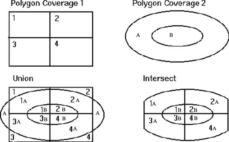
Polygon
Overlay: Intersect
In the QGIS Toolbox, find the 'Vector Overlay / Intersect' too. We will use this intersect option to create a new temparary layer. Here is the Procedure:
- We want to use the amesbuf layer as 'input layer' since we want to keep only the parts of the cambbgrp2010 block groups that are inside the buffer.
- cambbgrp2010.shp becomes the 'overlay layer'.
- We don't need to keep all the attribute fields in either layer. They will just clutter up the attribute table of the output. We don't need any fields from the amesbug layer and only the geoid10 identifier plus (from the cambbgrp2010 layer) the Area and the four columns with counts of persons by age from the Social Explorer spreadsheet. I chose to keep the STATEFP field from the input layer (amesbuf) and GEOID10, Area, and Perimeter in the overlay layer (cambbgrp2010). t
- When you are ready to run the intersection operation, the screen should look something like this:

The output is named 'Intersection' and will be added to your layer panel. Note that the layer includes only those parts of the block groups that were inside the Ames street buffer. Your screen should look something like this:

Take a look at the attribute table. Among the attribute fields is 'Area'. This column reports the original area of each blockgroup. Now, you need to add a new field that computes, for each block group that intersected the buffer, the area of that block group that falls within the buffer. Use the 'Field Calculator' icon on the attribute table window to add a field named, newarea, with data type 'decimal' and then compute the values in the column to be the '$area' variable in the Geometry list. Finally, add another new field called 'pct_inside' and calculate it to be newarea/Area. Toggle off the 'edit' icon (the pencil at the top left of the attribute table toolbar) and save your results. You now have, for each block group that intersects the Ames St. buffer, the proportion that is inside the buffer. Save this 'Intersection' temporary layer as a shapefile named, 'ames_bg_intersect', add it into your layer panel and remove the temporary 'Intersection' layer. The new fields in the attribute table of ames_bg_intersect should look something like this: (Note that this attribute table does not yet have the four columns from Social Explorer joined in)
Now we are ready to calculate our estimate of the number of children within the buffer age up to and including 17 years, adjusted for the relative portion of the block groups inside the buffer area. We are assuming that people are evenly distributed across each block group and hence the number of people falling within a buffer is proportional to the area of the polygon within the buffer area. Join the Social Explorer spreadsheet to cambbgrp2010 if you have not already done so. You may want to save cambbrgrp2010 into a new shapefile (which we call camb_bg_kids) so the joins are saved into a new shapefile before adding yet one more field. Then open the attribute table of camb_bg_kids and open the 'field calculator' window to add a new field for the count of kids under 18 who are estimated to live within the Ames St. buffer. once again and add a new first Click on the heading for "Popupto17" and use the Calculate Values menu item again to set:Popupto17 = ( [2009_13_15] + [2009_13_16] + [2009_13_17] + [2009_13_18]) * [Arearatio] Note: The field names may be changed when we did the intersect and/or joins so they are different than the field names in 009_13_ACS_Age_SocialExplorerTable.xls. DOUBLE CHECK your field names before performing the calculation. The intersect will maintain the order of your variables but not the names.
At this point, stop editing the table and save your results. Now you can use the 'selection' tools to calculate the sum of the estimates across all the block groups. This sum is your estimate of the number of children 17 or younger within 800 meters of Ames St. This is the answer to Question 3 of the lab assignment. Question 4 asks you to make a thematic map that documents your efforts.

Polygon
Overlay: Union
We could have done similar calculations using the union operation instead of intersection. Do you remember the difference. You need not redo all the calculations but tyr the union tool and/or do enough review of the tool description to understand the difference. Think about how union is different from intersect even though you can use either as a step toward the same end. Also pay attention to the number of features in your union file and think about which features do you want to include when running the summary option. Write your comments in the Question 5 section of the assignment.
Part
3: Other Spatial Analysis preparation tools (Optional)
-
Dissolving features and clipping layers
The above exercises only scratches the surface of spatial analysis tools in ArcGIS. We don't have time for more required exercises. This optional exercise focuses on two common operations:
- DISSOLVE - suppose we have a census block group map and we wish to create a census tract map. We can use the 'dissolve' tool to eliminate the block group boundaries that lie within a census tract.
- CLIP - this command acts like a cookie cutter.
For both these tools, appropriate handling of the feature attributes is the tricky part.
Assignment
Please use the assignment page to complete your assignment. You are asked to dp the following:
- Write a brief (few sentence) description of any interesting spatial pattern that you see for coffee shop locations within Cambridge.
- Create a labeled and annotated map supporting your description in Question 1.
- Estimate the number of children aged-17-and-under do who were living within 800 meters of Ames Street based on the 2010 census?
- Make a map showing Ames Street and the 800 m buffer on top of a block group thematic map showing children aged-17-and-under. Instead of mapping the 'number of children,' we suggest that you map the density of children in the original block groups. Do you see why? Label one of the larger block groups that partially overlaps your buffer with the percentage of the block group that is within 800 meters of Ames Street.
- Briefly describe the difference between the output layers (that is, the shapefiles) produced by using the union and intersect operations to combine your Ames street buffer with the Cambridge block groups.