Here is a summary of the R commands (after the initial installation of your local copy of 32-bit R) that we used in Lab Exercise #1 to read the BE, demographic, community type, and VMT data from our MS-Access database, do the principal component analysis, and ordinary least squares modeling:
| Step | R command |
| Load custom libraries | library("RODBC",lib.loc="C:\\TEMP\\Rlib32")
library("hexbin", lib="C:/temp/rlib32")
library("psych",lib.loc="C:\\TEMP\\Rlib32")
library("GPArotation",lib.loc="C:\\TEMP\\Rlib32")
|
| Open channel to MS-Access database | UAchannel <- odbcConnect("MS Access Database",uid="") |
| Read the 4 tables from MS-Access into R | demdata <- sqlFetch(UAchannel, "demographic_bg") bedata <- sqlFetch(UAchannel, "built_environment_250m") vmtdata <- sqlFetch(UAchannel, "vmt_250m") ctdata <- sqlFetch(UAchannel, "ct_grid") |
| Remove unwanted columns | outlist <- c("BG_ID","CT_ID","F1_wealth","F2_children","F3_working")
demdata2 <- demdata[,setdiff(names(demdata),outlist)]
demdata3 <- demdata2[demdata2[,'INC_MED_HS']>0,] |
| Remove rows if no income | demdata3 <- demdata2[demdata2[,'INC_MED_HS']>0,] |
| Remove incomplete rows | demdata4 <- demdata2[complete.cases(demdata2),] |
| Remove another column | outlist <- c("pct_ov2car")
demdata5 <-demdata4[,setdiff(names(demdata4),outlist)] |
| Find principal components | prin5 <- principal(demdata5, nfactors=3, rotate="varimax",scores=TRUE); |
| Get 4-way joined table from MS-Access | vmt_join <- sqlFetch(UAchannel, "t_vmt_join4") |
| Remove incomplete rows | vmtall <- vmt_join[complete.cases(vmt_join),] |
| Regress 9-cell VMT average on the 8 factors | run_ols1 <- lm(formula = (vmt_tot_mv / vin_mv) ~ f1_nw + f2_connect
+ f3_transit + f4_auto + f5_walk +f1_wealth
+ f2_kids + f3_work, data=vmtall) |
(1) Rerun these commands to be sure to start off with the same results as those we had at the end of the Tuesday session.
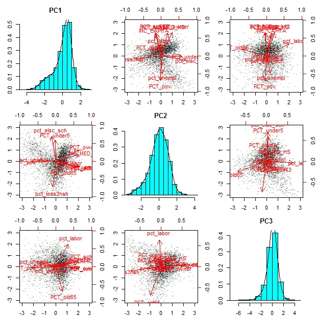
(2) Visualize the principal components that we identified (they are similar to the 3 demographic factors that Prof. Diao constructed). The histograms show the distribution of each component across all block groups. The scatterplots use pairs of the 3 components along the X-Y axes and superimpose the axes showing high/low directions for each of the original variables.
biplot(prin5)
(3) Let's examine the residuals from our ordinary least squares (OLS) model. These residuals are the actual values minus the values predicted by the regression model. We can use the residual function to extract the residuals from our regression model results and plot them against the relevant VMT estimate (which is ]vmt_tot_mv / vin_mv] for our model). The scatterplot works but has so many points that it is hard to interpret. To get a better visualization, use the 'hexbin' package.
- res1 <- resid(run_ols1)
- plot(vmtall$vmt_tot_mv / vmtall$vin_mv,res1,ylab="Residuals",xlab="VMT",main="Errors in VMT prediction")
- bin <- hexbin(vmtall$vmt_tot_mv / vmtall$vin_mv, res1)
- plot(bin,ylab="Residuals",xlab="VMT",main="Errors in VMT prediction")
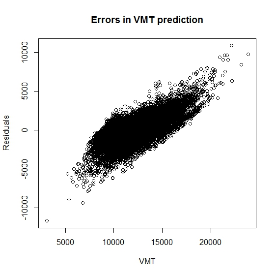
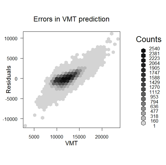
The scatterplots suggest that residuals and VMT are correlated - they are high or low together. This suggests that the adjustments to annual mileage that are associated with out factors may be better modeled as percentage changes rather than absolute value differences. With this in mind, we might consider fitting a model of log(VMT).
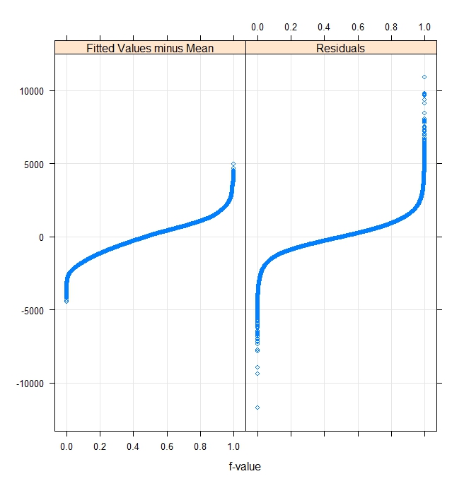
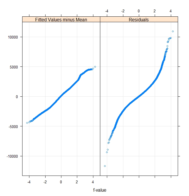
We might also want to use additional R tools to plot fitted values and residuals in order to check some of the model assumptions. The left quantile-quantile plot of fits and residuals assumes a uniform distribution and the right pair assumes a normal distribution. If the data follow the assumed distribution, then the plots will be linear. The fitted values look close to normal but the residuals are both widely varying and less normal.
rfs(run_ols1) |
rfs(run_ols1,distribution=qnorm) |
 |
 |
(4) Let's see if the residuals exhibit a different pattern within each community type. The community type is specified in one of the columns of 'vmtall'. We can stratify the block groups by community type and then examine the residuals for each group. To get the residuals into the same array as our original data, let's first add the residuals as an additional column to 'vmtall' - the large matrix used for our regression model. While we are at it, we use the fitted() function to pull the fitted values into a vector as well. We use the 'cbind' command (to combine columns) to merge the data, then we plot the residuals for each community type as a 'box and whiskers plot'
- fit1 <- fitted(run_ols1)
- vmtall2 <- cbind(vmtall,fit1,res1)
- boxplot(res1 ~ ct, data=vmtall2,ylab="Residuals",main="VMT Residuals by Community Type")
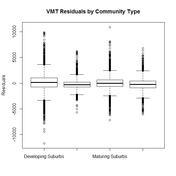
The median and interquartile range are fairly similar but their might be some heteroscedasticity since the residuals seem to be much larger in the developing suburbs than in the inner core (the second column). Also, the inner core has a negative median residual suggesting that city cars tend to be driven even less than the model would suggest.
(5) Next, let's move some of the R results into MS-Access tables so we can get them into ArcGIS for spatial analysis and mapping. R provides functions that can save our data objects so we do not have to recreate them every time. We can save data in R's native format or move specific data arrays into external tables as plain text files or tables in a database manager such as MS-Access. The following commands save vmtall2 in R's format (indicated by the Rdata suffix), as a CSV text file, and as a table called 'vmtall2' in MS-Access. We also save in R format the three original tables that we imported from MS-Access.
- save(vmtall2,file="c:/temp/data_ua/rdata/vmtall2.rdata")
- save(bedata,file="c:/temp/data_ua/rdata/bedata.rdata")
- save(demdata,file="c:/temp/data_ua/rdata/demdata.rdata")
- save(vmtdata,file="c:/temp/data_ua/rdata/vmtdata.rdata")
- write.csv(vmtall2,file="c:/temp/data_ua/rdata/vmtall2b.csv",row.names=FALSE) ## do not add row numbers to the output
- sqlSave(UAchannel, vmtall2, rownames=FALSE)
Use Windows Explorer and MS-Access to check that these files and tables are written into the expected location.
There are many ways to save and retrieve data in R. Use help(save) to look into the variations. Sometimes, it is helpful to save your entire R workspace so that you can pick up where you left off, and the command save.image() bundles a particular flavor of save() options in order to do this. However, you may have trouble with save.image() on lab machines since you do not have write permission for certain default locations. Also, your workspace may includes external connections such as your channel to MS-Access. You are left on your own to review the help files and experiment with various 'save' options to find the variation of 'save' that works best for you.
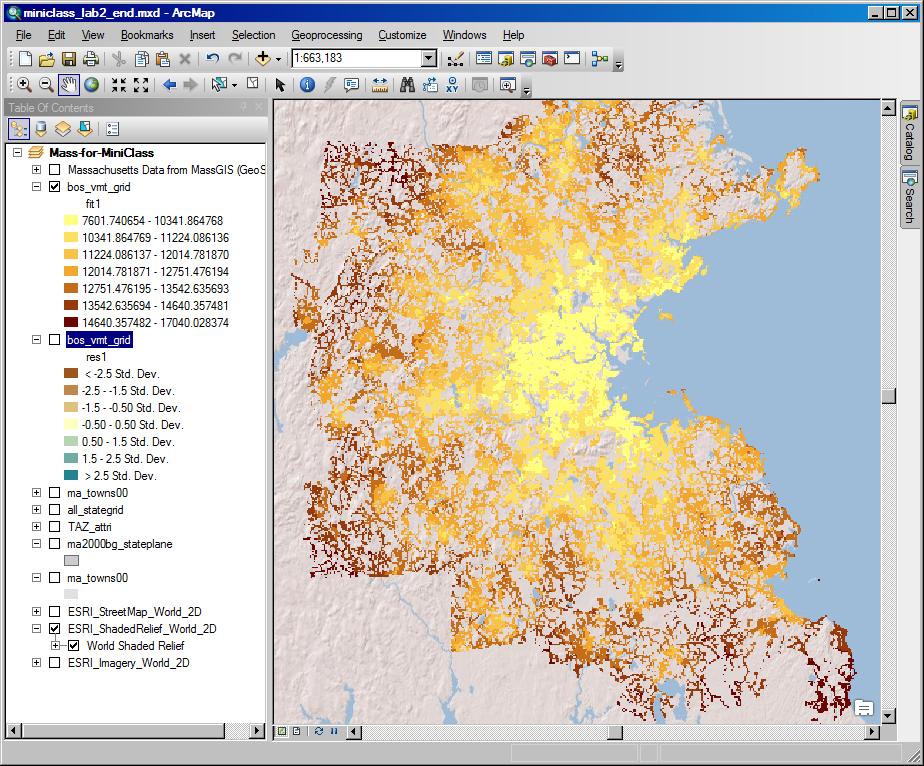
(6) Examining the model results in ArcMap: If you have not already done so, find and double-click on the saved ArcMap document in c:\temp\data_ua\miniclass_lab2start.mxd to open the shapefiles for the MiniClass:

Click the 'add data' icon, navigate to your MS-Access database and add the 'vmtall2' table that we just create in R. Join this table to the 'all_stategrid' shapefile based on the grid cell ID, 'g250m_id'. Say 'yes' when asked about creating an index. Next, create a thematic map of the residuals from our OLS model (res1) and classify the data by 'standard deviation' so we can easily spot with high/med/low residuals. The red cells with high residuals are the places where the model underestimated the actual VMT. At this point, you will notice that the map takes a long time to redraw. This is because there are 356K grid cells in Massachusetts - but only 53250 have estimates (because they were in metro Boston and met the criteria regarding VINs, households, and estimated annual mileage). To speed up the processing, you may want to create a new shapefile, bos_vmt_grid.shp, with only those 53250 grid cells that have data. You will also want to set the grid cell outline color to 'none' so the boundaries do not obscure the shading. When you set the thematic shading in the classification window, click the 'sampling' button and change the maximum sample size to be 54000. Otherwise, the breakpoints for the shading will be determine only using the first 10000 grid cells. Finally, we have added two web mapping services (one from MassGIS and three from ESRI). You can turn these on to overlay images, road maps and shaded relief maps in order to help you interpret metro Boston areas at different scales. The result for the fitted values and the residuals should look something like this:
 |
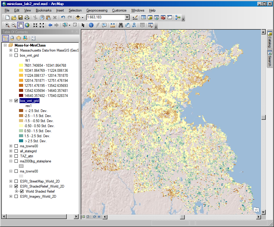 |
Take advantage of having the vmtall2 table joined to the all_stategrid to examine other thematic maps of factor values, fitted VMT values, and the like. From the plot of residuals, it does look like some spatial patterns have been missed. The residuals are way negative (i.e., red - implying that we overestimated mileage) for inner core grid cells and it looks like they are also low for some of the regional centers and transportation corridors. Alternatively, the residuals are relatively high (blue) for some of the suburban grid cells that are mixed in with the 'null' grid cells (where no one lives because it is a pond or open space). These impressions may help us think of additional factors or relationships that could capture some of the remaining spatial effects. For your convenience, the above ArcMap document has been saved as the miniclass_lab2_end.mxd in the 'data_ua' sub-directory of the class locker. The newly created bos_vmt_grid.shp shapefile has also been added to the 'shapefile' folder within the 'data_ua' sub-directory of the class locker so the ArcMap document can find this new shapefile. Be aware, however, that the 'vmtall2' table that we generated in R has not been added to the MS-Access database saved in the class locker. Finally, we also save the ArcMap document in version 10.0 format as, miniclass_lab2_end_v10.0.mxd in case some of you are still running ArcGIS ver. 10.0 on your personal machines.
(7) Open the ArcMap help files and search for spatial autocorrelation - that is, the extent to which a spatial pattern is non-random. You may want to look at the Introduction to the ArcGIS Geostatistical Analyst Tutorial. At least read about 'how spatial autocorrelation (Moran's I) works'. You may want to try some of the geostatistical tools to in the spatial statistics section to examine the nature and extent of spatial autocorrelation in the data.
(8) A popular free tool for analyzing spatial autocorrelation is Open GeoDa (developed by Lou Anselin, et al., now at Arizona State). Some of his tools are integrated into ArcGIS. We do not have GeoDa loaded on the lab machines, but you can download your own copy from here:
- Home page: https://geodacenter.asu.edu/
- Download site: https://geodacenter.asu.edu/software/downloads
You can use this tool to read shapefiles such as the bos_vmt_grid.shp that you just created and do spatial statistics. If you have time, load the package onto your personal machine and try it out on bos_vmt_grid.