17.2 Combined Conduction and Convection
We can now analyze problems in which both conduction and convection
occur, starting with a wall cooled by flowing fluid on each side. As
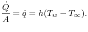
discussed, a description of the convective heat transfer can be
given explicitly as
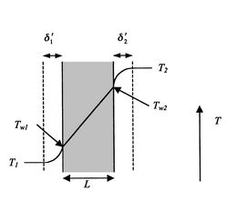
This could represent a model of a turbine blade with internal
cooling. Figure 17.6 shows the configuration.
Figure 17.6:
Conducting wall with convective
heat transfer
|
|
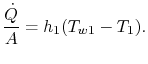
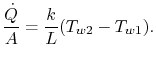
The heat transfer in fluid 1 is given by
which is the heat transfer per unit area to the fluid. The heat
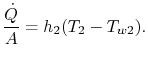
transfer in fluid 2 is similarly given by
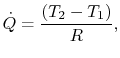
Across the wall, we have
The quantity  is the same in all of these expressions.
Putting them all together to write the known overall temperature
drop yields a relation between heat transfer and overall temperature
drop,
is the same in all of these expressions.
Putting them all together to write the known overall temperature
drop yields a relation between heat transfer and overall temperature
drop,  :
:
![$\displaystyle T_2-T_1 = (T_2-T_{w2})+(T_{w2}-T_{w1})+(T_{w1}-T_1) =\frac{\dot{Q}}{A}\left[\frac{1}{h_1}+\frac{L}{k}+\frac{1}{h_2}\right].$](img2022.png) |
(17..20) |
We can define a thermal resistance,  , as before, such that
where
is given by
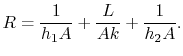 |
(17..21) |
Equation (17.21) is the thermal resistance for a
solid wall with convection heat transfer on each side.
For a turbine blade in a gas turbine engine, cooling is a critical
consideration. In terms of Figure 17.6,  is
the combustor exit (turbine inlet) temperature and
is
the combustor exit (turbine inlet) temperature and  is the
temperature at the compressor exit. We wish to find
is the
temperature at the compressor exit. We wish to find  because
this is the highest metal temperature. From
(17.20), the wall temperature can be written
as
because
this is the highest metal temperature. From
(17.20), the wall temperature can be written
as
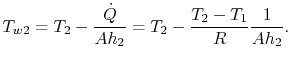 |
(17..22) |
Using the expression for the thermal resistance, the wall
temperatures can be expressed in terms of heat transfer coefficients
and wall properties as
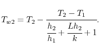 |
(17..23) |
Equation (17.23) provides some basic design
guidelines. The goal is to have a low value of
. This means
 should be large,
  should be large (but we may not have
much flexibility in choice of material) and
should be large (but we may not have
much flexibility in choice of material) and  should be small. One
way to achieve the first of these is to have
should be small. One
way to achieve the first of these is to have  low (for example,
to flow cooling air out as in
Figure 17.1 to shield the
surface).
low (for example,
to flow cooling air out as in
Figure 17.1 to shield the
surface).
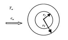
A second example of combined conduction and convection is given by a
cylinder exposed to a flowing fluid. The geometry is shown in
Figure 17.7.
Figure 17.7:
Cylinder in a flowing fluid
|
|
For the cylinder the heat flux at the outer surface is given by
The boundary condition at the inner surface could be
either a heat flux condition or a temperature specification; we use
the latter to simplify the algebra. Thus,  at
at  . This
is a model for the heat transfer in a pipe of radius
. This
is a model for the heat transfer in a pipe of radius  surrounded by insulation of thickness
  . The solution for
a cylindrical region was given in
Section 16.5.1 as
. The solution for
a cylindrical region was given in
Section 16.5.1 as
Use of the boundary condition
 yields
  .
.
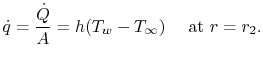
At the interface between the cylinder and the fluid,  , the
temperature and the heat flow are continuous. (Question: Why is
this? How would you argue the point?)
, the
temperature and the heat flow are continuous. (Question: Why is
this? How would you argue the point?)
![$\displaystyle \dot{q} = \underbrace{-k\frac{dT}{dr}}_{\substack{\textrm{heat fl...
...2}{r_1}\right)+T_1\right)-T_\infty\right]} _\textrm{surface heat flux to fluid}$](img2033.png) |
(17..24) |
Plugging the form of the temperature distribution in the cylinder
into Equation (17.24) yields
The constant of integration,  , is
, is
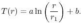
and the expression for the temperature is, in normalized
non-dimensional form,
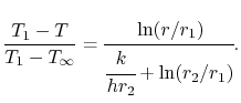 |
(17..25) |
The heat flow per unit length,  , is given by
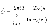 |
(17..26) |
The units in Equation (17.26) are W/m-s.
A problem of interest is choosing the thickness of insulation to
minimize the heat loss for a fixed temperature difference
 between the inside of the pipe and the flowing fluid far
away from the pipe. (
is the driving temperature
distribution for the pipe.) To understand the behavior of the heat
transfer we examine the denominator in
Equation (17.26) as
between the inside of the pipe and the flowing fluid far
away from the pipe. (
is the driving temperature
distribution for the pipe.) To understand the behavior of the heat
transfer we examine the denominator in
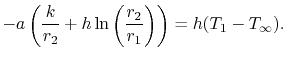
Equation (17.26) as  varies. The thickness
of insulation that gives maximum heat transfer is given by
varies. The thickness
of insulation that gives maximum heat transfer is given by
 |
(17..27) |
(Question: How do we know this is a maximum?)
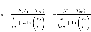
From Equation (17.27), the value of
for maximum
is thus
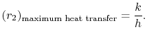 |
(17..28) |
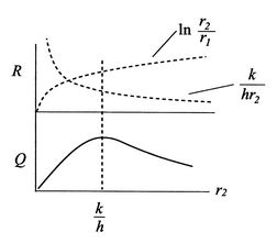
If
is less than this, we can add insulation and
increase heat loss. To understand why this occurs, consider
Figure 17.8, which shows a
schematic of the thermal resistance and the heat transfer. As
increases from a value less than  , two effects take
place. First, the thickness of the insulation increases, tending to
drop the heat transfer because the temperature gradient decreases.
Secondly, the area of the outside surface of the insulation
increases, tending to increase the heat transfer. The second of
these is (loosely) associated with the
, two effects take
place. First, the thickness of the insulation increases, tending to
drop the heat transfer because the temperature gradient decreases.
Secondly, the area of the outside surface of the insulation
increases, tending to increase the heat transfer. The second of
these is (loosely) associated with the  term, the first with
the
term, the first with
the
 term. There are thus two competing effects
which combine to give a maximum
at
.
term. There are thus two competing effects
which combine to give a maximum
at
.
Figure 17.8:
Critical radius of insulation
|
|
Muddy Points
In the expression  , what is
  ? (MP 17.4)
It seems that we have simplified convection a lot. Is finding the
heat transfer coefficient,  , really difficult?
(MP 17.5)
, really difficult?
(MP 17.5)
What does the ``K'' in the contact resistance formula stand for?
(MP 17.6)
In the equation for the temperature in a cylinder
(17.25), what is ``r?''
(MP 17.7)
UnifiedTP
|