Thermodynamics and Propulsion

18.1 Temperature Distributions in the Presence of Heat Sources

There are a number of situations in which there are sources of heat in the domain of interest. Examples are:

1. Electrical heaters where electrical energy is converted resistively into heat.
2. Nuclear power supplies.
3. Propellants where chemical energy is the source.

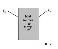
These situations can be analyzed by looking at a model problem of a slab with heat sources $\alpha$ (W/m³) distributed throughout. We take the outside walls to be at temperature $T_w$ and we will determine the maximum internal temperature.

Figure 18.1: Slab with heat sources

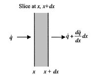
[Overall configuration] [Infinitesimal slice]

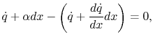
With reference to Figure 18.1(b), a steady-state energy balance yields an equation for the heat flux, $\dot{q}$ :

$$\dot{q} + \alpha dx - \left(\dot{q}+\frac{d\dot{q}}{dx}dx\right)=0,$$

or

$$\frac{d\dot{q}}{dx}=\alpha.$$

There is a change in heat flux with $x$ due to the presence of the heat sources. The equation for the temperature is

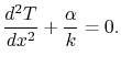$$\frac{d^2T}{dx^2} +\frac{\alpha}{k} = 0.$$ (18..1)

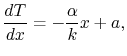
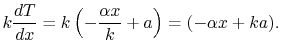
Equation (18.1) can be integrated once,

$$\frac{dT}{dx} = -\frac{\alpha}{k}x + a,$$

and again to give

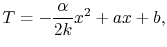$$T = -\frac{\alpha}{2k}x^2 +a x + b,$$ (18..2)

where $a$ and $b$ are constants of integration. The boundary conditions imposed are $T(0)= T(L) = T_w$ . Substituting these into Equation (18.2) gives $b =T_w$ and $a = \alpha L/2k$ . The temperature distribution is thus

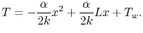$$T = -\frac{\alpha}{2k}x^2 +\frac{\alpha}{2k}L x + T_w.$$ (18..3)

Writing (18.3) in a normalized, non-dimensional fashion gives a form that exhibits in a more useful manner the way in which the different parameters enter the problem:

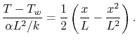$$\frac{T-T_w}{\alpha L^2/k} = \frac{1}{2}\left(\frac{x}{L}-\frac{x^2}{L^2}\right).$$ (18..4)

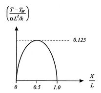
Figure 18.2: Temperature distribution for slab with distributed heat sources

This distribution is sketched in Figure 18.2. It is symmetric about the mid-plane at $x = L/2$ , with half the energy due to the sources exiting the slab on each side.

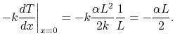
The heat flux at the side of the slab, $x = 0$ , can be found by differentiating the temperature distribution and evaluating at $x = 0$ :

$$-k\frac{dT}{dx}\biggr\vert _{x=0} = - k\frac{\alpha L^2}{2 k}\frac{1}{L} = -\frac{\alpha L}{2}.$$

This is half of the total heat generated within the slab. The magnitude of the heat flux is the same at $x = L$ , although the direction is opposite.

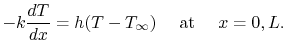
A related problem would be one in which there were heat flux (rather than temperature) boundary conditions at $x = 0$ and $x = L$ , so that $T_w$ is not known. We again determine the maximum temperature. At $x = 0$ and $L$ , the heat flux and temperature are continuous so

$$-k\frac{dT}{dx} = h(T-T_\infty)\quad\textrm{ at }\quad x=0,L.$$ (18..5)

Referring to the temperature distribution of Equation (18.2) gives for the two terms in Equation (18.5),

$$k\frac{dT}{dx} = k\left(-\frac{\alpha x}{k}+a\right)=(-\alpha x + k a).$$

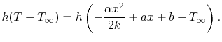$$h(T-T_\infty) = h\left(-\frac{\alpha x^2}{2k}+a x + b - T_\infty\right).$$ (18..6)

Evaluating (18.6) at $x = 0$ and $L$ allows determination of the two constants $a$ and $b$ . This is left as an exercise for the reader.

Muddy Points

For an electric heated strip embedded between two layers, what would the temperature distribution be if the two side temperatures were not equal? (MP 18.1)