Magnetic field gradients, magnetization gratings and k-space

In order to record an image of a sample (or obtain other spatial information) there must be a measurable difference introduced between two locations in the sample. The most straightforward approach to this is to apply a magnetic field gradient,

,

so that the resonance frequency varies across the sample.

Only the three partial derivatives of the z-component of the magnetic field are of interest, since the others correspond to static fields in the transverse direction of the laboratory frame, and thus rotating fields in the rotating frame. Rotating fields (with respect to the spin) do not influence the long time spin dynamics.

The presence of a magnetic field gradient introduces a spatial heterogeneity into the experiment so that the resonance frequency varies over the sample.

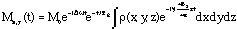
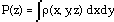
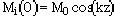
Recall that the observed signal is the integrated bulk magnetization from the entire sample. If a z-gradient (_Bz/_z) is applied to a sample whose spin density is described by r(x,y,z) then the FID, is,

.

This is put in a more recognizable form by introducing the reciprocal space vector,

,

and by defining the projection of the spin density along the z-axis,

,

so that,

,

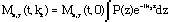
where Mx,y(t,0) is the NMR signal in the absence of the magnetic field gradient. The measured NMR signal in the presence of a magnetic field gradient is the Fourier transform of the projection of the spin density along the direction of the gradient convoluted with the NMR lineshape in the absence of the gradient,

.

It is helpful to understand how it is that the NMR signal is a measure of the Fourier components of the spin density. As shown above, spin evolution in the presence of a magnetic field gradient introduces a sinusoidal magnetization grating across the sample and the k-vector describes the spacing of the grating,

,

where lz is the period of the grating.

The above figure shows the modulation of M_y for a cylindrical sample in a transverse gradient as a function of time, or k.

The essence of the NMR imaging experiment is that by a suitable combination of magnetic field gradients oriented along the x, y, and z laboratory frame directions any Fourier component of the spin density can be measured. Since these gradients are under experimental control and can be switched on in a time very short compared to the NMR relaxation times, then there is a great deal of flexibility in how one proceeds to record all of the necessary Fourier components needed to reconstruct an image. We will return to this after discussing the limits to resolution, and multiple-pulse experiments (see lecture 4).

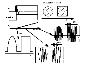
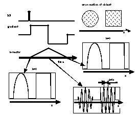
A schematic description of a one-dimensional NMR imaging experiment to measure the projection of the object spin density along a given axis. The object is shown and consists of two regions of spins with circular and square cross sections. The z-axis is identified and the applied magnetic field gradient is a _Bz/_z gradient, so the Larmor frequency of the spins in the object increases from left to right. The measurement is proceeded by an RF pulse that excites the spins and places them in the transverse plane. The three profiles of the object show one axis of the transverse magnetization at three different values of k. Higher k values correspond to finer magnetization gratings. The NMR signal is the integrated spin magnetization across the sample which for this sample has the shape shown following the RF pulse.

Above, the NMR image is described as a convolution of a spatial function describing the density of the spins, and a frequency function describing the NMR spectrum. To make sense of this, the NMR spectrum must be converted into spatial units. Notice that in the presence of a constant magnetic field gradient, the two reciprocal space vectors, time and k, are directly proportional to each other,

.

So if the NMR spectrum corresponds to a single resonance line (such is the case for water) then the image resolution can be described in terms of the linewidth, nfwhm, (or the spin-spin relaxation time) and the gradient strength,

.

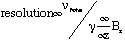Sharper lines and stronger gradients lead to higher resolution. This is what makes NMR imaging of solids challenging since the T2 is approximately 1000 times shorter for solids than for liquids.

The above movie shows a repeat of the spatial encoding shown earlier but here attenuation due to spin-spin relaxation is included. The grating decays as, exp(-k/(g G T₂)), where T₂ = 1 m s and G = 1 Gauss. Notice that at fine gratings the modulation no longer fills the entire object.

There are other limitations to the obtainable resolution, the most important in microscopy of liquids being the random molecular motions of the spins. Water has a diffusion coefficient of about 3 µm2/ms at room temperature, and as the molecules move they carry their magnetic moment with them. This leads to an irreversible blurring of the magnetization grating and hence a loss in high spatial frequency information. The influence of the spin's motion on the magnetization grating is included in the Bloch Eq. by adding a diffusion term,

.

In a constant grating,

,

and as the molecules move the overall action is an attenuation of this grating,

,

where A is a real number.

,

or

.

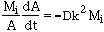This has solutions of,

,

so the magnetization decays as,

in a constant grating, and

in a constant magnetic field gradient. The factor three in the exponential of the final expression arises since the spacing of the grating varies with time, and the attenuation is most pronounced for finer gratings.

The above movie shows a repeat of the spatial encoding shown earlier but here attenuation due to molecular diffusion is included. Notice that compared to the attenuation from the spin-spin relaxation term, diffusion is only pronounced at fine gratings.

That the various interactions, gradient, chemical shift, susceptibility, couplings, each drive the spin dynamics individually is useful and permits a simple linear model of the imaging system's sensitivity and resolution, but equally important (particularly in creating contrast) is the experimenter's ability to separate these by selectively refocusing one or more interactions. The gradient echo is perhaps the simplest example of this. Recall that the periodicity of the magnetization grating is the zero moment of the time-dependent gradient waveform (the integrated area of the waveform. By applying the gradient as a bi-polar pulse pair (see the following figure) the grating is removed from the object at the end of the gradient waveform and the spins are re-focused (back in phase).

A gradient echo is generated by a bi-polar gradient waveform. Since the k-vector is the integrated area under the gradient waveform at the end of the bi-polar gradient k returns to zero, and there is no magnetization grating across the sample. At the mid-point of the gradient waveform k is maximum and the grating is at its finest. Since the NMR signal is the integration of the spin magnetization across the sample, the signal maximums correspond to the two points where k is zero, and hence an echo is observed.

Since the only interaction that is influenced by the presence of a gradient is the gradient evolution itself, the bipolar gradient waveform shown in the figure will not refocus the chemical shift, or any other internal interaction. We will leave the applications of gradient echoes to the next lecture. Here we make the point, that the gradient echo may be employed to observe the extent of attenuation due to molecular diffusion.