1.6
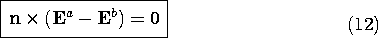
Faraday's Integral Law
The laws of Gauss and Ampère relate fields to sources. The statement of charge conservation implied by these two laws relates these sources. Thus, the previous three sections either relate fields to their sources or interrelate the sources. In this and the next section, integral laws are introduced that do not involve the charge and current densities.
Faraday's integral law states that the circulation of E around a contour C is determined by the time rate of change of the magnetic flux linking the surface enclosed by that contour (the magnetic induction).
As in Ampère's integral law and Fig. 1.4.1, the right-hand rule relates ds and da.
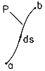
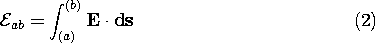
Figure 1.6.1. Integration line for definition of electromotive force. The electromotive force, or EMF, between points (a) and (b) along the path P shown in Fig. 1.6.1 is defined as
We will accept this definition for now and look forward to a careful development of the circumstances under which the EMF is measured as a voltage in Chaps. 4 and 10.
Electric Field Intensity with No Circulation
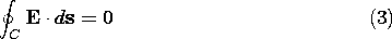
First, suppose that the time rate of change of the magnetic flux is negligible, so that the electric field is essentially free of circulation. This means that no matter what closed contour C is chosen, the line integral of E must vanish.
We will find that this condition prevails in electroquasistatic systems and that all of the fields in Sec. 1.3 satisfy this requirement.
Illustration. A Field Having No Circulation
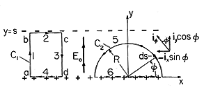
A static field between plane parallel sheets of uniform charge density has no circulation. Such a field, E = Eo ix, exists in the region 0 < y < s between the sheets of surface charge density shown in Fig. 1.6.2. The most convenient contour for testing this claim is denoted C1 in Fig. 1.6.2.
Figure 1.6.2. Uniform electric field intensity Eo, between plane parallel uniform distributions of surface charge density, has no circulation about contours C1 and C2. Along path 1, E
ds = Eo dy, and integration from y = 0 to y = s gives sEo for the EMF of point (a) relative to point (b). Note that the EMF between the plane parallel surfaces in Fig. 1.6.2 is the same regardless of where the points (a) and (b) are located in the respective surfaces.
On segments 2 and 4, E is orthogonal to ds, so there is no contribution to the line integral on these two sections. Because ds has a direction opposite to E on segment 3, the line integral is the integral from y = 0 to y = s of E
4 In setting up the line integral on a contour such as 3, which has a direction opposite to that in which the coordinate increases, it is tempting to double-account for the direction of ds not only be recognizing that ds = -iy dy, but by integrating from y = s to y = 0 as well.In this planar geometry, a field that has only a y component cannot be a function of x without incurring a circulation. This is evident from carrying out this integration for such a field on the rectangular contour C1. Contributions to paths 1 and 3 cancel only if E is independent of x.
Example 1.6.1. Contour Integration
To gain some appreciation for what it means to require of E that it have no circulation, no matter what contour is chosen, consider the somewhat more complicated contour C2 in the uniform field region of Fig. 1.6.2. Here, C2 is composed of the semicircle (5) and the straight segment (6). On the latter, E is perpendicular to ds and so there is no contribution there to the circulation.
On segment 5, the vector differential ds is first written in terms of the unit vector i
, and that vector is in turn written (with the help of the vector decomposition shown in the figure) in terms of the Cartesian unit vectors.
It follows that on the segment 5 of contour C2
and integration gives
So for contour C2, the circulation of E is also zero.
When the electromotive force between two points is path independent, we call it the voltage between the two points. For a field having no circulation, the EMF must be independent of path. This we will recognize formally in Chap. 4.
Electric Field Intensity with Circulation
The second limiting situation, typical of the magnetoquasistatic systems to be considered, is primarily concerned with the circulation of E, and hence with the part of the electric field generated by the time-varying magnetic flux density. The remarkable fact is that Faraday's law holds for any contour, whether in free space or in a material. Often, however, the contour of interest coincides with a conducting wire, which comprises a coil that links a magnetic flux density.
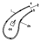
Illustration. Terminal EMF of a Coil
A coil with one turn is shown in Fig. 1.6.3. Contour (1) is inside the wire, while (2) joins the terminals along a defined path. With these contours constituting C, Faraday's integral law as given by (1) determines the terminal electromotive force. If the electrical resistance of the wire can be regarded as zero, in the sense that the electric field intensity inside the wire is negligible, the contour integral reduces to an integration from (b) to (a).
5 With the objectives here limited to attaching an intuitive meaning to Faraday's law, we will give careful attention to the conditions required for this terminal relation to hold in Chaps. 8, 9, and 10.In view of the definition of the EMF, (2), this integration gives the negative of the EMF. Thus, Faraday's law gives the terminal EMF as
Figure 1.6.3. Line segment (1) through a perfectly conducting wire and (2) joining the terminals (a) and (b) form closed contour.
where
f, the total flux of magnetic field linking the coil, is defined as the flux linkage. Note that Faraday's law makes it possible to measure
oH electrically (as now demonstrated).
Demonstration 1.6.1. Voltmeter Reading Induced by Magnetic Induction
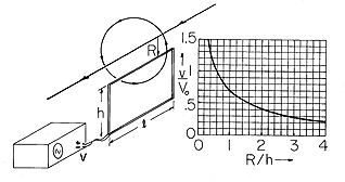
The rectangular coil shown in Fig. 1.6.4 is used to measure the magnetic field intensity associated with current in a wire. Thus, the arrangement and field are the same as in Demonstration 1.4.1. The height and length of the coil are h and l as shown, and because the coil has N turns, it links the flux enclosed by one turn N times. With the upper conductors of the coil at a distance R from the wire, and the magnetic field intensity taken as that of a line current, given by (1.4.10), evaluation of (8) gives
Figure 1.6.4. Demonstration of voltmeter reading induced at terminals of a coil in accordance with Faraday's law. To plot data on graph, normalize voltage to Vo as defined with (11). Because I is the peak current, v is the peak voltage. In the experiment, the current takes the form
where
= 2
(60). The EMF between the terminals then follows from (8) and (9) as
A voltmeter reads the electromotive force between the two points to which it is connected, provided certain conditions are satisfied. We will discuss these in Chap. 8.
In a typical experiment using a 20-turn coil with dimensions of h = 8 cm, l = 20 cm, I = 6 amp peak, the peak voltage measured at the terminals with a spacing R = 8 cm is v = 1.35 mV. To put this data point on the normalized plot of Fig. 1.6.4, note that R/h = 1 and the measured v/Vo = 0.7.


 E , J
E , J  o E
o E