The permanent magnetization model of Sec. 9.3 is a somewhat artificial example of the magnetization density M specified, independent of the magnetic field intensity. Even in the best of permanent magnets, there is actually some dependence of M on H.
Constitutive laws relate the magnetization density M or the magnetic flux density B to the macroscopic H within a material. Before discussing some of the more common relations and their underlying physics, it is well to have in view an experiment giving direct evidence of the constitutive law of magnetization. The objective is to observe the establishment of H by a current in accordance with Ampère's law, and deduce B from the voltage it induces in accordance with Faraday's law.
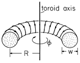
Figure 9.4.1 Toroidal coil with donut-shaped magnetizable core.
Example 9.4.1. Toroidal Coil
A coil of toroidal geometry is shown in Fig. 9.4.1. It consists of a donut-shaped core filled with magnetizable material with N1 turns tightly wound on its periphery. By means of a source driving its terminals, this coil carries a current i. The resulting current distribution can be assumed to be so smooth that the fine structure of the field, caused by the finite size of the wires, can be disregarded. We will ignore the slight pitch of the coil and the associated small current component circulating around the axis of the toroid.
Because of the toroidal geometry, the H field in the magnetizable material is determined by Ampère's law and symmetry considerations. Symmetry about the toroidal axis suggests that H is
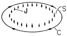
directed. The integral MQS form of Ampère's law is written for a contour C circulating about the toroidal axis within the core and at a radius r. Because the major radius R of the torus is large compared to the minor radius
w, we will ignore the variation of r over the cross-section of the torus and approximate r by an average radius R. The surface S spanned by this contour and shown in Fig. 9.4.2 is pierced N1 times by the current i, giving a total current of N1 i. Thus, the azimuthal field inside the core is essentially
Note that the same argument shows that the magnetic field intensity outside the core is zero.
Figure 9.4.2 Surface $S$ enclosed by contour C used with Ampère's integral law to determine H in the coil shown in Fig. 9.4.1. In general, if we are given the current distribution and wish to determine H, recourse must be made not only to Ampère's law but to the flux continuity condition as well. In the idealized toroidal geometry, where the flux lines automatically close on themselves without leaving the magnetized material, the flux continuity condition is automatically satisfied. Thus, in the toroidal configuration, the H imposed on the core is determined by a measurement of the current i and the geometry.
How can we measure the magnetic flux density in the core? Because B appears in Faraday's law of induction, the measurement of the terminal voltage of an additional coil, having N2 turns also wound on the donut-shaped core, gives information on B. The terminals of this coil are terminated in a high enough impedance so that there is a negligible current in this second winding. Thus, the H field established by the current i remains unaltered.
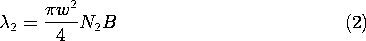
The flux linked by each turn of the sensing coil is essentially the flux density multiplied by the cross-sectional area
w2/4 of the core. Thus, the flux linked by the terminals of the sensing coil is
and flux density in the core material is directly reflected in the terminal flux-linkage.
The following demonstration shows how (1) and (2) can be used to infer the magnetization characteristic of the core material from measurement of the terminal current and voltage of the first and second coils.
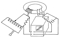
Demonstration 9.4.1. Measurement of B-H Characteristic
The experiment shown in Fig. 9.4.3 displays the magnetization characteristic on the oscilloscope. The magnetizable material is in the donut-shaped toroidal configuration of Example 9.4.1 with the N1-turn coil driven by a current i from a Variac. The voltage across a series resistance then gives a horizontal deflection of the oscilloscope proportional to H, in accordance with (1).
Figure 9.4.3 Demonstration in which the B-H curve is traced out in the sinusoidal steady state. The terminals of the N2 turn-coil are connected through an integrating network to the vertical deflection terminals of the oscilloscope. Thus, the vertical deflection is proportional to the integral of the terminal voltage, to
, and hence through (2), to B.
In the discussions of magnetization characteristics which follow, it is helpful to think of the material as comprising the core of the torus in this experiment. Then the magnetic field intensity H is proportional to the current i, while the magnetic flux density B is reflected in the voltage induced in a coil linking this flux.
Many materials are magnetically linear in the sense that
Here
m is the magnetic susceptibility. More commonly, the constitutive law for a magnetically linear material is written in terms of the magnetic flux density, defined by (9.2.8).
According to this law, the magnetization is taken into account by replacing the permeability of free space
o by the permeability
Typical susceptibilities for certain elements, compounds, and common materials are given in Table 9.4.1. Most common materials are only slightly magnetizable. Some substances that are readily polarized, such as water, are not easily magnetized. Note that the magnetic susceptibility can be either positive or negative and that there are some materials, notably iron and its compounds, in which it can be enormous. In establishing an appreciation for the degree of magnetizability that can be expected of a material, it is helpful to have a qualitative picture of its microscopic origins, beginning at the atomic level but including the collective effects of groups of atoms or molecules that result when they become as densely packed as they are in solids. These latter effects are prominent in the most easily magnetized materials.
TABLE 9.4.1RELATIVE SUSCEPTIBILITIES OF COMMON MATERIALS
Material PARAMAGNETIC Mg 1.2 x 10⁻⁵ Al 2.2 x 10⁻⁵ Pt 3.6 x 10⁻⁴ air 3.6 x 10⁻⁷ O2 2.1 x 10⁻⁶ DIAMAGNETIC Na -0.24 x 10⁻⁵ Cu -1.0 x 10⁻⁵ diamond -2.2 x 10⁻⁵ Hg -3.2x 10⁻⁵ H2O -0.9 x 10⁻⁵ FERROMAGNETIC Fe (dynamo sheets) 5.5 x 10³ Fe (lab specimens) 8.8 x 10⁴ Fe (crystals) 1.4 x 10⁶ Si-Fe transformer sheets 7 x 10⁴ Si-Fe crystals 3.8 x 10⁶ 105 FERRIMAGNETIC Fe3O4 100 ferrites 5000 The magnetic moment of an atom (or molecule) is the sum of the orbital and spin contributions. Especially in a gas, where the atoms are dilute, the magnetic susceptibility results from the (partial) alignment of the individual magnetic moments by a magnetic field. Although the spin contributions to the moment tend to cancel, many atoms have net moments of one or more Bohr magnetons. At room temperature, the orientations of the moments are mostly randomized by thermal agitation, even under the most intense fields. As a result, an applied field can give rise to a significant magnetization only at very low temperatures. A paramagnetic material displays an appreciable susceptibility only at low temperatures.
If, in the absence of an applied field, the spin contributions to the moment of an atom very nearly cancel, the material can be diamagnetic, in the sense that it displays a slightly negative susceptibility. With the application of a field, the orbiting electrons are slightly altered in their circulations, giving rise to changes in moment in a direction opposite to that of the applied field. Again, thermal energy tends to disorient these moments. At room temperature, this effect is even smaller than that for paramagnetic materials.
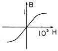
At very low temperatures, it is possible to raise the applied field to such a level that essentially all the moments are aligned. This is reflected in the saturation of the flux density B, as shown in Fig. 9.4.4. At low field intensity, the slope of the magnetization curve is
Figure 9.4.4 Typical magnetization curve without hysteresis. For typical ferromagnetic solids, the saturation flux density is in the range of 1-2 Tesla. For ferromagnetic domains suspended in a liquid, it is .02-.04 Tesla. Until now, we have been considering the magnetization of materials that are sufficiently dilute so that the atomic moments do not interact with each other. In solids, atoms can be so closely spaced that the magnetic field due to the moment of one atom can have a significant effect on the orientation of another. In ferromagnetic materials, this mutual interaction is all important.
To appreciate what makes certain materials ferromagnetic rather than simply paramagnetic, we need to remember that the electrons which surround the nuclei of atoms are assigned by quantum mechanical principles to layers or "shells." Each shell has a particular maximum number of electrons. The electron behaves as if it possessed a net angular momentum, or spin, and hence a magnetic moment. A filled shell always contains an even number of electrons which are distributed spatially in such a manner that the total spin, and likewise the magnetic moment, is zero.
For the majority of atoms, the outermost shell is unfilled, and so it is the outermost electrons that play the major role in determining the net magnetic moment of the atom. This picture of the atom is consistent with paramagnetic and diamagnetic behavior. However, the transition elements form a special class. They have unfilled inner shells, so that the electrons responsible for the net moment of the atom are surrounded by the electrons that interact most intimately with the electrons of a neighboring atom. When such atoms are as closely packed as they are in solids, the combination of the interaction between magnetic moments and of electrostatic coupling results in the spontaneous alignment of dipoles, or ferromagnetism. The underlying interaction between atoms is both magnetic and electrostatic, and can be understood only by invoking quantum mechanical arguments.
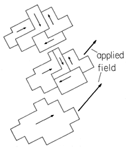
In a ferromagnetic material, atoms naturally establish an array of moments that reinforce. Nevertheless, on a macroscopic scale, ferromagnetic materials are not necessarily permanently magnetized. The spontaneous alignment of dipoles is commonly confined to microscopic regions, called domains. The moments of the individual domains are randomly oriented and cancel on a macroscopic scale.
Macroscopic magnetization occurs when a field is applied to a solid, because those domains that have a magnetic dipole moment nearly aligned with the applied field grow at the expense of domains whose magnetic dipole moments are less aligned with the applied field. The shift in domain structure caused by raising the applied field from one level to another is illustrated in Fig. 9.4.5. The domain walls encounter a resistance to propagation that balances the effect of the field.
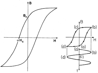
Figure 9.4.5 Polycrystalline ferromagnetic material viewed at the domain level. In the absence of an applied magnetic field, the domain moments tend to cancel. (This presumes that the material has not been left in a magnetized state by a previously applied field.) As a field is applied, the domain walls shift, giving rise to a net magnetization. In ideal materials, saturation results as all of the domains combine into one. In materials used for bulk fabrication of transformers, imperfections prevent the realization of this state. A typical trajectory traced out in the B-H plane as the field is applied to a typical ferromagnetic material is shown in Fig. 9.4.6. If the magnetization is zero at the outset, the initial trajectory followed as the field is turned up starts at the origin. If the field is then turned down, the domains require a certain degree of coercion to reduce their average magnetization. In fact, with the applied field turned off, there generally remains a flux density, and the field must be reversed to reduce the flux density to zero. The trajectory traced out if the applied field is slowly cycled between positive and negative values many times is the one shown in the figure, with the remanence flux density Br when H = 0 and a coercive field intensity Hc required to make the flux density zero. Some values of these parameters, for materials used to make permanent magnets, are given in Table 9.4.2.
TABLE 9.4.2 MAGNETIZATION PARAMETERS FOR PERMANENT MAGNET
Material Hc (A/m) Br (Tesla) Carbon steel 4000 1.00 Alnico 2 43,000 0.72 Alnico 7 83,500 0.70 Ferroxdur 2 143,000 0.34
Figure 9.4.6 Magnetization characteristic for material showing hysteresis with typical values of Br and Hc given in Table 9.4.2. The curve is obtained after many cycles of sinusoidal excitation in apparatus such as that of Fig. 9.4.3. The trajectory is traced out in response to a sinusoidal current, as shown by the inset. In the toroidal geometry of Example 9.4.1, H is proportional to the terminal current i. Thus, imposition of a sinusoidally varying current results in a sinusoidally varying H, as illustrated in Fig. 9.4.6b. As the i and hence H increases, the trajectory in the B-H plane is the one of increasing H. With decreasing H, a different trajectory is followed. In general, it is not possible to specify B simply by giving H (or even the time derivatives of H). When the magnetization state reflects the previous states of magnetization, the material is said to be hysteretic. The B-H trajectory representing the response to a sinusoidal H is then called the hysteresis loop.
Hysteresis can be both harmful and useful. Permanent magnetization is one result of hysteresis, and as we illustrated in Example 9.3.2, this can be the basis for the storage of information on tapes. When we develop a picture of energy dissipation in Chap. 11, it will be clear that hysteresis also implies the generation of heat, and this can impose limits on the use of magnetizable materials.
Liquids having significant magnetizabilities have been synthesized by permanently suspending macroscopic particles composed of single ferromagnetic domains. Here also the relatively high magnetizability comes from the ferromagnetic character of the individual domains. However, the very different way in which the domains interact with each other helps in gaining an appreciation for the magnetization of ferromagnetic polycrystalline solids.
In the absence of a field imposed on the synthesized liquid, the thermal molecular energy randomizes the dipole moments and there is no residual magnetization. With the application of a low frequency H field, the suspended particles assume an average alignment with the field and a single-valued B-H curve is traced out, typically as shown in Fig. 9.4.4. However, as the frequency is raised, the reorientation of the domains lags behind the applied field, and the B-H curve shows hysteresis, much as for solids.
Although both the solid and the liquid can show hysteresis, the two differ in an important way. In the solid, the magnetization shows hysteresis even in the limit of zero frequency. In the liquid, hysteresis results only if there is a finite rate of change of the applied field.
Ferromagnetic materials such as iron are metallic solids and hence tend to be relatively good electrical conductors. As we will see in Chap. 10, this means that unless care is taken to interrupt conduction paths in the material, currents will be induced by a time-varying magnetic flux density. Often, these eddy currents are undesired. With the objective of obtaining a highly magnetizable insulating material, iron atoms can be combined into an oxide crystal. Although the spontaneous interaction between molecules that characterizes ferromagnetism is indeed observed, the alignment of neighbors is antiparallel rather than parallel. As a result, such pure oxides do not show strong magnetic properties. However, a mixed-oxide material like Fe3O4 (magnetite) is composed of sublattice oxides of differing moments. The spontaneous antiparallel alignment results in a net moment. The class of relatively magnetizable but electrically insulating materials are called ferrimagnetic.
Our discussion of the origins of magnetization began at the atomic level, where electronic orbits and spins are fundamental. However, it ends with a discussion of constitutive laws that can only be explained by bringing in additional effects that occur on scales much greater than atomic or molecular. Thus, the macroscopic B and H used to describe magnetizable materials can represent averages with respect to scales of domains or of macroscopic particles. In Sec. 9.5 we will make an artificial diamagnetic material from a matrix of "perfectly" conducting particles. In a time-varying magnetic field, a magnetic moment is induced in each particle that tends to cancel that being imposed, as was shown in Example 8.4.3. In fact, the currents induced in the particles and responsible for this induced moment are analogous to the induced changes in electronic orbits responsible on the atomic scale for diamagnetism[1].