Deadlines
Useful links
lab3.py -- testing code for Lab #3
channel.py -- channel code (same as previous labs)
lab3_1.py -- template for Task #1
lab3_4.py -- template for Task #4
lab3_6.py -- optional template for Task #6
lab3.zip -- zip file containing all of the above
Numpy docs,
tutorial,
examples
Matplotlib.pyplot
reference,
tutorial
Goal
In this lab we'll look into what happens when noise is added to the signal as it propagates from transmitter to receiver. We'll develop a mathematical model for noise, investigate how best to sample a noisy signal, and measure the number of bit errors caused by noise.
This lab also includes a design problem, where you will use the insights you have gained about noise and about LTI systems to design a system that will transmit data across the IR channel using as few samples per bit as you can. For the design problem, you will probably need a working scaled_ir class (Task 4 from Lab2). If you do not have a working version of scaled_ir, or need other functions from Lab 2, talk with your TA.
Instructions
See Lab #1 for a longer narrative about lab mechanics. The 1-sentence version:
Complete the tasks below, submit your task files on-line before the deadline, and sign-up for your check-off interview with your TA.
As always, help is available in 32-083 (see the Lab Hours web page), and we are doing our best to try to provide more help during peak hours.
Task 1: Computing sample statistics (1 point)
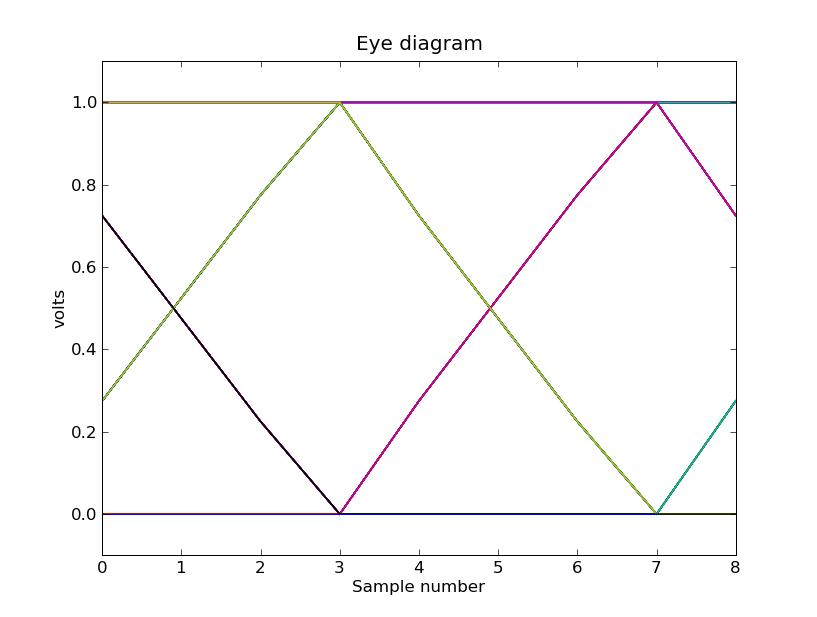
In Lab 2, Task #1, we plotted eye diagrams for signals after they had passed through a channel. Below is an eye diagram generated by transmitting a random sequence of bits across noise-free channel that limits the speed of transitions. For this channel, the inter-symbol interference extends only to one adjacent bit when 4 or more samples/bit are used. In the following eye diagram, 4 samples were used per bit (making the bit period four samples long), and the transmitted samples were equal to 1.0 volt when a '1' bit was being transmitted, and the transmitted samples were 0.0 volts when a '0' bit was being transmitted.
If we choose a digitization threshold of 0.5V, we can see that in this noiseless example we could successfully sample this signal using any sample numbered 0 mod 4, 2 mod 4, or 3 mod 4 -- i.e., only if we tried to sample the signal at samples numbered 1 mod 4 would we make mistakes in determining which bit the transmitter intended to send. But to make the comparison with the digitization threshold as easy as possible, it would be best to choose the sample where the eye is most "open" -- samples numbered 3 mod 4 in this case.
As a first step in automating the process of determining where to sample, consider the following diagram which shows how the sample voltages are distributed at each of the four sample times within a bit period. In the histogram for each of the four sample times, the length of the line indicates the fraction of samples that have the indicated voltage value.
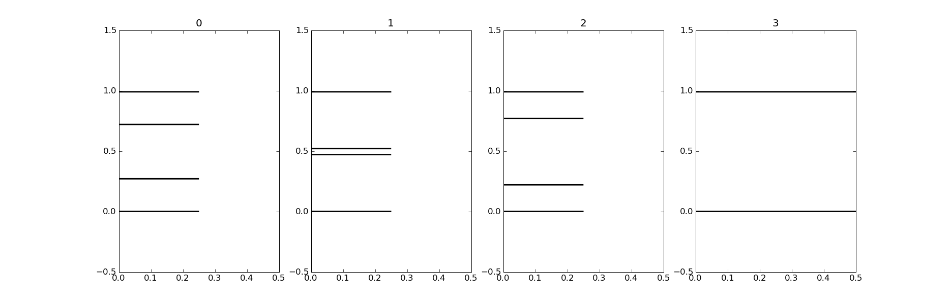
At sample times 0, 1 and 2 the samples are divided evenly among four possible intermediate voltages; at sample 3 the samples are divided evenly between the two final voltages 0.0V and 1.0V.
Following the usual modus operandi, let's write a function to compute some statistics for each possible sample time given a particular channel. lab3_1.py is the template file for this task:
# this is the template for Lab #3, Task #1
import numpy
import matplotlib.pyplot as p
import lab3
reload(lab3)

p.ion()

def sample_stats(samples,samples_per_bit=4,vth=0.5):
    # reshape array into samples_per_bit columns by as many
    # rows as we need.  Each column represents one of the
    # sample times in a bit period.
    bins = numpy.reshape(samples,(-1,samples_per_bit))

    # now compute statistics each column
    stats = []
    for i in xrange(samples_per_bit):
        column = bins[:,i]
        dist = column - vth  # subtract vth from each sample
        min_dist = ??? # Your code here
        avg_dist = ??? # Your code here
        avg_squared_dist = ??? # Your code here
        stats.append((min_dist,avg_dist,avg_squared_dist))

    return stats  # return collected statistics

if __name__ == '__main__':
    stats = sample_stats(lab3.channel_data)
    for i in xrange(len(stats)):
        min,avg,avgsq = stats[i]
        print "sample %d: min_dist=%6.3f, avg_dist=%6.3f, " \
              "avg_squared_dist=%6.3f" % (i,min,avg,avgsq)

    # when ready for checkoff, enable the following line
    #lab3.checkoff(sample_stats,'L3_1')
Finish the sample_statistics function given in the template so that for each of the possible sample times within a bit period it prints the following:
When you're satisfied with your implementation, enable the call to lab3.checkoff which will submit your code on-line.
There are some lab questions (see link at top of page) associated with this task.
Task 2: Modeling channel noise (1 point)
In lecture we learned that noise in transmission channels is actually the sum of a myriad of small perturbances, each of which has a value randomly chosen independently from a uniform distribution (where each value in the interval of possible values is equally likely to occur).
Let's run an experiment to get some idea of how noise values might be statistically distributed. Experiments using repeated random sampling are called Monte Carlo methods, named after the famous casino. Suppose that channel noise comes from 100,000 sources each of which contributes a voltage independently chosen from a uniform distribution in the range -0.001V to +0.001V. In a uniform distribution, all the probabilities are equal.
Some useful functions:
Write a Python function channel_noise that produces a noise value computed using the parameters above (100,000 sources, each contributing a value chosen from a uniform distribution in the range -0.001V to +0.001V).
Call channel_noise 10,000 times and produce a histogram of the results. You might want to start with, say, 100 calls to channel_noise until you are producing the histogram correctly. As we learned in lecture, we'd expect to find the results looking like a Gaussian distribution.
As it turns out (cf. Central Limit Theorem), we would get a Gaussian distribution for the total noise no matter what distribution we chose for the individual independent contributions as long as the distribution has a finite expected value and a finite variance.
There are some lab questions (see link at top of page) associated with this task.
Task 3: Sampling in the presence of noise (1 point)
If we now add some noise to each channel (randomly chosen from the Gaussian distribution explored in Task #2) and plot the sample distribution, the figure from Task #1 now looks like
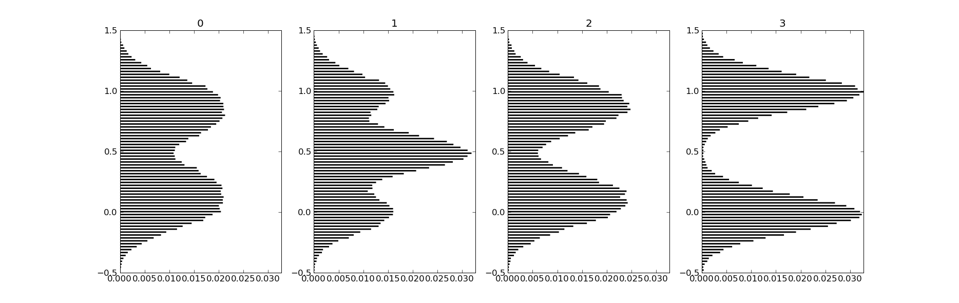
With noise, at each sample time we no longer see a sample distribution that only has samples at a small number of voltages -- each of the lines in the Task #1 histogram has been replaced by a Gaussian distribution centered where the lines used to be.
Rerun your code from Task #1, this time calling sample_stats with the argument lab3.noisy_channel_data. Think about the results and select the statistic you'll use to determine which sample number corresponds to the most open part of the eye.
There are some lab questions (see link at top of page) associated with this task.
Task 4: Experimentally determining the bit error rate (2 points)
In circumstances like the IR channel, where the time between samples is large (0.25 microseconds) compared to the accuracy of a crystal-based time reference (typically tens to hundreds of picoseconds), one can asssume an essentially fixed bit period. Given that assumption, converting a sequence of received samples in to a sequence of received bits can be accomplished by
1) reshaping the received samples in to a sample array, where a sample array is a matrix with samples_per_bit columns and (number-of-received-samples)/(samples_per_bit) rows,
2) selecting the column of the sample array that corresponds to the widest open part of the eye in an eye diagram, using a suitable statistic,
3) comparing each element of the selected column to a threshold, and generating an associated '1' bit when the threshold is exceeded, and a '0' bit if not.
In this task you will be estimating bit error rates on a noisy instantiation of the slow channel by sending 10,000 bit long random messages through the channel and determining what percentage of the bits arrive correctly. As will be described below, you will be asked to write the functions that determine the appropriate column of the sample array to use for bit conversion, to write the function that computes the estimate of the bit error rate.
In order to use the slow channel channel, it is necessary to deal with uncertain delays in the channel (as you saw in Lab 1). Since you have already dealt with this synchronization problem in Lab 1 and in Lab 2, we have written a template for this task that will generate a 10,000 bit random message, surround the message with padding, prepend the message with a 10-bit synchronization sequence, and strip off the synchronization sequence from the received bits. Since you will be dealing with noisy channels, there will be bit errors, and sometimes the bit errors will be in the synchronization sequence. If there is a bit error in the synchronization sequence, our function fails (with an appropriate error message), and you should just run it again. PLEASE NOTE: bit errors in the synchronization sequence should only occur occasionally (once every 5-10 runs). If your are getting the error message more frequently than that, there is probably a bug in your implementation of the following functions. Also, try running the program several times. The results will be a little different each time because of the randomness of noise. All you will need to add to the lab3_4.py template is an implementation of two functions: receive and bit_error_rate. Based on your deliberations in Task #3, write a Python function receive that returns a numpy array of message bits given a numpy array of samples produced by the channel:
Also write a Python function bit_error_rate that compares a numpy array of transmitted bits to a numpy array of received bits and returns the fraction of bit locations that don't match. For example, if two 1000-element bit sequences mismatch in two bit locations, the result would be 2/1000 = .002.
# this is the template for Lab #3, Task #4
import matplotlib.pyplot as p
import math,numpy,random
import channel
reload(channel)
import lab3
reload(lab3)
import lab1
reload(lab1)
import lab1_1
reload(lab1_1)


# Takes a numpy array of samples, a number of samples per bit, and a
# threshold for turning a selected sample from each bit period in 0
# bit or a 1 bit. Returns a numpy array of the bits.
def receive(samples,samples_per_bit,vth):
    """
    Apply a statistical measure to samples to determine which
    sample in the bit period should be used to determine the
    transmitted message bit.  vth is the digitization threshold.
    Return a numpy array of received message bits.
    """
    pass # your code here

# Compares two numpy arrays of bits (0's and 1's),
# return percentage mismatch
def bit_error_rate(seq1,seq2):
    """
    Perform a bit-by-bit comparison of two numpy arrays of bits,
    returning the fraction of mismatches.
    """
    pass # your code here


# Sends bits through the channel, receive, remove sync and return bits.
def xmit_and_rcv(bits, mychannel, samples_per_bit, sync):

    # Convert the bits to samples
    samples = lab1.bits_to_samples(bits,samples_per_bit=samples_per_bit)

    # Now send through the chane
    noisy_data = mychannel(samples)

    # Truncate received date to ensure an integral number of bit periods
    noisy_data = noisy_data[0:len(noisy_data) -
                              len(noisy_data)%samples_per_bit]

    # Use the average of the min and max as the threshold.
    vth = 0.5*(numpy.max(noisy_data) + numpy.min(noisy_data))
    #print "vth", vth

    # Call your receive function with numpy array of received noisy data
    rcvd = receive(noisy_data,samples_per_bit,vth)

    # Yank off the sync, here's that convolution trick again.
    # Why is the sync reversed before the convolution.  Why didn't we
    # do that with the mark in lab2 task 4?  (Hint: symmetry).
    zero_centered_sync = sync[::-1] - 0.5  # Reverse and 0.5='1', -0.5='0'
    convolved_with_rcvd = numpy.convolve(zero_centered_sync, rcvd)
    max_conv = numpy.max(convolved_with_rcvd)
    start_index = numpy.nonzero(convolved_with_rcvd == max_conv)[0][0]

    # Get the rcvd data after the sync
    rcvd = rcvd[start_index+1:]

    return rcvd

if __name__ == '__main__':

    # Noise standard deviation
    noise = 0.2

    # bits of leading and trailing zeros as padding.
    pad_bits = 10

    # A start of transmission sync byte.
    sync_seq = [1,1,0,0,0,0,0,1,0,1]

    # Pick channel one with the given noise, with Gaussian
    # (normal) distrib.
    mychannel = channel.channel(channelid='1',
                                noise=noise,
                                use_normal=True)

    # Generate 10,000 random bits
    bit_seq = [random.randint(0,1) for i in xrange(10000)]

    # Generate bit sequence with a start sync, plus lead and trail
    # padding. Turn sequences into numpy arrays for ease of processing
    # later.
    bit_seq_pad = [0]*pad_bits + [1]*pad_bits + \
                  sync_seq + bit_seq + [0]*pad_bits
    sbits = numpy.array(bit_seq_pad)
    sync = numpy.array(sync_seq)
    bits = numpy.array(bit_seq)

    for samples_per_bit in [200,50]:

        # Send bits through the channel, receive, remove sync
        # and return bits.
        rcvd = xmit_and_rcv(sbits, mychannel, samples_per_bit, sync)

        # Eliminate trailing bits
        rcvd = rcvd[0:len(bits)]

        # Check that enough bits were received
        lr = len(rcvd)
        ls = len(bits)
        assert lr==ls,"Number of rcvd bits=%d, " \
                      "Number of sent bits=%d.\n" \
                      "Probably you were unlucky and had a " \
                      "bit error in the sync bits.\n" \
                      "Try running again." % (lr,ls)

        # Finally, use your procedure to compute the percentage of
        # bit errors, or bit error rate, of rcvd bits.
        ber = bit_error_rate(bits, rcvd)

        print "bit error rate = %g for %d samples/bit."  % \
              (ber,samples_per_bit)

    # when ready for checkoff, enable the following line
    #lab3.checkoff(bit_error_rate,'L3_4')
When you're satisfied with your implementation, enable the call to lab3.checkoff which will submit your code on-line.
There are some lab questions (see link at top of page) associated with this task.
Task 5: Computing the bit error rate (2 points)
Using some of the ideas from lecture we can derive an analytic estimate for the bit-error rate. In the experiments above we've been trying to determine the transmitted message bit by choosing samples from each bit period where the eye was most open. Looking at the eye diagram associated with the channel in Task #1, we can see that at sample 3 in the transmission of each bit, the expected sample voltage in a noise-free environment is 0.0V if we're transmitting a "0" bit and 1.0V if we're transmitting a "1" bit. For the more realistic channel '1' used in Task #4, when the number of samples_per_bit is high enough (as is the case when samples_per_bit = 200), we can make a similar statement. That is, there will be a sample in each bit period whose voltage in a noise-free environment will be 0.0V if we're transmitting a "0" bit and 1.0V if we're transmitting a "1" bit. NOTE: This is not the case if samples_per_bit = 50!
Now let's consider what happens when the channel adds noise to the signal. We'll get an error (i.e., receive a bit incorrectly) if there's sufficient noise so that the received sample falls on the wrong side of the threshold. For example, the transmission of a "1" would be received in error if
transmitted_voltage + noise_voltage ≤ threshold voltage
which is satisfied if the noise voltage &le -0.5V assuming we set the digitization threshold at 0.5V. Similarly, a transmitted "0" would be received in error if the noise voltage at that sample was ≥ 0.5V.
We can use these observations to develop a formula for the probability of a reception error based on the probability of the noise voltage at that sample being larger or smaller than a certain amount:
p(error) = p(transmitted "1" received as "0") +
           p(transmitted "0" received as "1")

         = p(transmitted a "1") * p(noise ≤ -0.5) +
           p(transmitted a "0") * p(noise ≥ +0.5)

         = 0.5*p(noise ≤ -0.5) + 0.5*p(noise ≥ 0.5)
where we've used the information that we're transmitting a random bit stream so the probability of transmitting a "1" or a "0" is 1/2.
That just leaves figuring out the probabilities of the noise voltage being ≤ -0.5V or ≥ 0.5V. We've argued that the probability distribution function (PDF) for the noise is Gaussian, so the two probabilities we want are the shaded areas in the figure below.
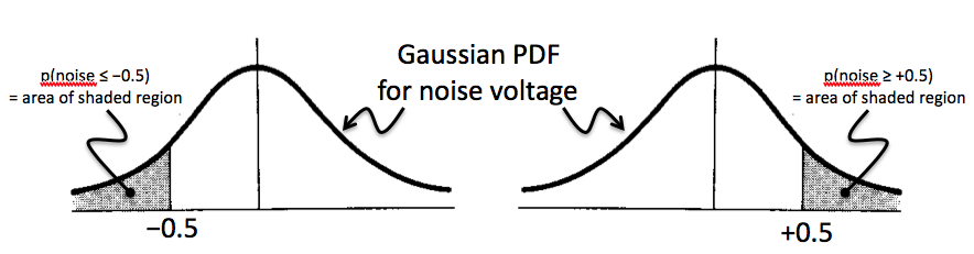
The area of the shaded regions can be determined from the cumulative distribution function (CDF) for the noise, defined for a value x as the integral of the PDF from -∞ to x, i.e., the probability that a value chosen according the PDF is ≤ x. So the area of the shaded area on the left is just the value of the CDF at -0.5, and, noting that the total area under the PDF is 1, the value of the shaded area on the right is 1 minus the value of the CDF at +0.5.
lab3.py includes the lab3.unit_normal_cdf(x) function which computes the value of the CDF at x for a unit normal PDF, i.e., a Gaussian PDF with a mean of 0 and a standard deviation of 1. The noise PDF used in this lab also has a mean of 0, but its standard deviation is 0.2 (set by the noise parameter in the channel instantiation), so we can't use lab3.unit_normal_cdf directly. But it's easy scale our argument (y) to one that can be used via the following formula:
x = (y - mean_of_y)/standard_deviation_of_y
Complete the calculation for p(error) using the formulas above and calls to lab3.unit_normal_cdf to come up with a numerical estimate for expected bit-error rate.
First compare your analytic calculation to the bit error rates computed in Task #4 for the samples_per_bit = 200 case. The two results should agree with each other fairly closely (the bit error rates should be with twenty percent of each other). We computed a result of approximately 0.006.
Once you have agreement between your analytic and experimental bit error rate computations for the samples_per_bit = 200 case, consider the samples_per_bit=50 case in Task #4. In this second case, you will have to consider intersymbol interference (ISI). To compute the correct bit error rate, you will have to examine the associated eye diagram for a noise-free version of channel '1' (use your lab2 Task 1 function). From the eye diagram, you can determine the noise-free values for the possible voltages at the sample used for bit detection. Please refer to the annotated lecture notes for Lecture 5 if you need a reminder of how to compute bit error rates in the case of ISI. If your analytic and experimental bit error rate calculations are both correct, they should match to within twenty percent.
There are some lab questions (see link at top of page) associated with this task.
Task 6, a design problem, (3 points)
THIS DESIGN TASK USES THE IR HARDWARE! MAKE SURE YOU USE THE 6.02 VERSIONS OF IDLE, AND PLEASE BE SURE NOT TO PUT THE REFLECTOR ANY CLOSER TO THE IR HARDWARE THAN SIX INCHES AWAY. OTHERWISE, YOU WILL SATURATE THE RECEIVERS AND LOSE ANY LINEARITY!
In the ealier tasks, you used software models of three transmission channels to learn about modeling, and compensating for, the impact of channel behavior on transmitted data. In addition, you developed a scaled_ir channel that makes the IR hardware channel look like a linear time-invariant system. Finally, you computed the unit sample response for the scaled_ir system, and demonstrated that the unit sample response could be convolved with complicated inputs and accurately predict the scaled_ir channel's output.
For this design task, please start with your solution for Task 4 of Lab 2, and your solution to Task 4 of this lab, though change the length of the random bit sequence from 10,000 to 500 (to save time). Then develop a post-processed IR channel that can transfer bits using as few samples per bit as you can manage, with zero errors, at least for the 500 bit sequence.
If you plan to use deconvolution (a sensible strategy since it works so well for the software channels), then you will soon discover that using deconvolution on the IR system by directly using the unit sample response computed in Lab 2, Task #4 is (almost certainly unless you are very lucky) a disaster.
There are many ways of resolving the deconvolution difficulties, and one possible strategy is to suitably manipulate the unit sample response USR) computed in Lab 2, Task #4 before using the USR in deconvolution. If you decide to try such a strategy, think about what you know about unit sample and unit step responses, and think about what you learned from lecture and from answering the problem set question on deconvolution.
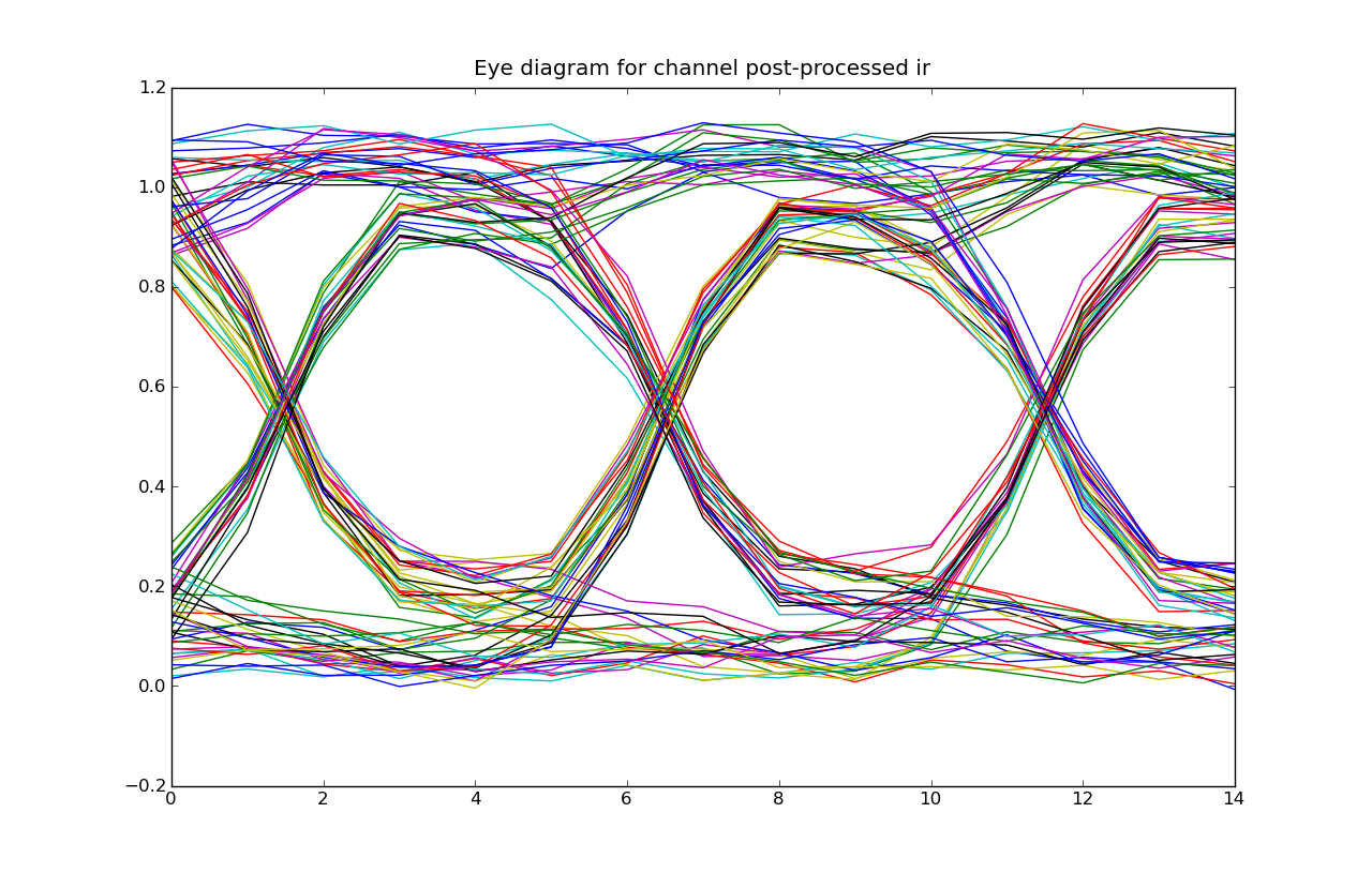
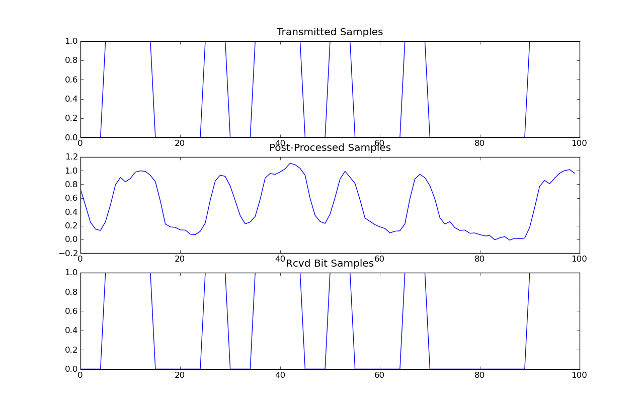
To demonstrate the performance of your design, have your test code create figures like the ones below showing the eye diagram for your post-processed IR channel and the results returned by your processed scaled_ir and the recovered message bits. Your test code should also compare the transmitted and received message and report how many errors were detected. Here's a figure from a solution that achieves error-free transmission with rate of just 5 samples/bit when the flourescent lights (a major source of IR noise) are off:
You are welcome to do this design problem any way you like, but we have also provided a template that it set up for solving this problem using deconvolution with a modified unit sample response (though you will have determine the modification to the unit sample response by modifying the function modify_h )
lab3_6.py -- Possible Template for task #6
If you are ambitious, see how well your post-processed IR channel works when the reflector is moved further from the IR hardware, or if you expose the channel to room flouresent light.