Useful links
Numpy docs,
tutorial,
examples
Matplotlib.pyplot
reference,
tutorial
Goal
In this lab we'll measure what happens when we transmit information over real-world (non-ideal) channels, build a mathematical model of the channel, and then use it to improve receiver performance. We'll introduce eye diagrams as a useful tool for visualing what happens to signals as they pass through a channel.
Instructions
See Lab #1 for a longer narrative about lab mechanics. The 1-sentence version:
Complete the tasks below, submit your task files on-line before the deadline, and complete your check-off interview within a week of the file submission deadline.
As always, help is available in 32-083 (see the Lab Hours web page).
Task 1: Generating useful test sample sequences (1 point)
In order to run experiments on transmitting data through various channels, we'll need a handy way to construct test sample sequences. Please write a Python function transmit that generates the sequence of voltage samples output by the transmitter given a sequence of message bits to be sent:
voltage_samples = transmit(bits,npreamble=0,
                                npostamble=0,
                                samples_per_bit=8,
                                v0 = 0.0,
                                v1 = 1.0,
                                repeat = 1)
npreamble -- number of "0" samples to output before any of the message bits are transmitted. See v0 keyword arg for value to be used.
npostamble -- number of "0" samples to output after all the message bits have been transmitted. See v0 keyword arg for value to be used.
samples_per_bit -- how many voltage samples to output for each message bit. So total number of samples output for one repitition is npreamble + samples_per_bit*len(bits) + npostamble.
v0 -- floating point voltage to use when generating samples for "0" bits (repeated samples_per_bit times).
v1 -- floating point voltage to use when generating samples for "1" bits (repeated samples_per_bit times).
repeat -- an integer specifying how many times to repeat the sequence of preamble samples, message samples, and postamble samples.
The default value for each keyword argument (i.e., the value used if the caller doesn't explicitly specify a value) is chosen so that no keyword arguments need be supplied unless the user is trying to do something out of the ordinary.
lab2_1.py is a template for your Task #1 design file:
# template for Lab #2, Task #1
import lab2

def transmit(bits,npreamble=0,
             npostamble=0,
             samples_per_bit=8,
             v0 = 0.0,
             v1 = 1.0,
             repeat = 1):
    """ generate sequence of voltage samples:
          bits: binary message sequence
          npreamble: number of leading v0 samples
          npostamble: number of trailing v0 samples
          samples_per_bit: number of samples for each message bit
          v0: voltage to output for 0 bits
          v1: voltage to output for 1 bits
          repeat: how many times to repeat whole shebang
    """
    pass  # your code here...

if __name__ == '__main__':
    # give the transmit function a workout, report errors
    lab2.test_transmit(transmit)
The call to lab2.test_transmit will try calling your function and verify that the sample sequence it returns is correct. If the test detects an error, a diagnostic message describing the failure is printed; if no errors are detected, no message is printed and the test routine simply returns.
Task 2: Sending data streams through a channel (1 point)
In lab2.py we've provided two functions that compute the effect of transmitting a sequence of voltage samples through each of two channels:
receive_samples = lab2.channel1(transmit_samples,noise=0.0)
receive_samples = lab2.channel2(transmit_samples,noise=0.0)
Just ignore the noise keyword argument for now.
Write a Python function test_channel that plots the result of sending some test sample sequences through the channel function passed as an argument:
Please use the same ranges for the vertical axes in both plots to make it easy to compare the two sample sequences (the horizontal axes will be the same since there are the same since the output sequence will have the same number of samples as the input sequence). This means you'll need to set the ranges programmatically (using matplotlib.pyplot.axis) to override the auto-ranging built into the plot routines -- call axis after you've plotted the values. Choose the appropriate plot ranges intelligently by determining the minimum and maximum values to be plotted -- just don't use some hard-wired constants that happen to work for these particular channels.
As always, the plots and axes should have meaningful labels. Note that you can get the name of the channel function using channel.__name__. You might also find matplotlib.pyplot.subplots_adjust a useful function to get the subplot spacing the way you want it.
lab2_2.py is a template file for this task:
# template for Lab #2, Task #2
import matplotlib.pyplot as p
import lab2

# turn on interactive mode, useful if we're using ipython
p.ion()

def test_channel(channel):
    """
    create a test waveform and plot both it and the output of
    passing the waveform through the channel.
    """
    pass  # your code here

if __name__ == '__main__':
    # try out our two channels
    test_channel(lab2.channel1)
    test_channel(lab2.channel2)

    # interact with plots before exiting.  p.show() returns
    # after all plot windows have been closed by the user.
    # Not needed if using ipython
    p.show()
Interview questions:
Task 3: Determining the unit-sample response of a channel (1 point)
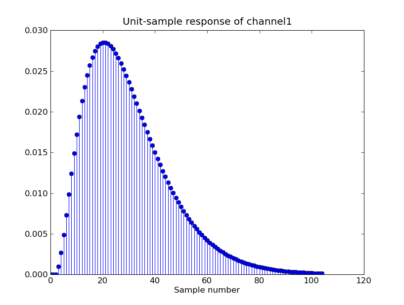
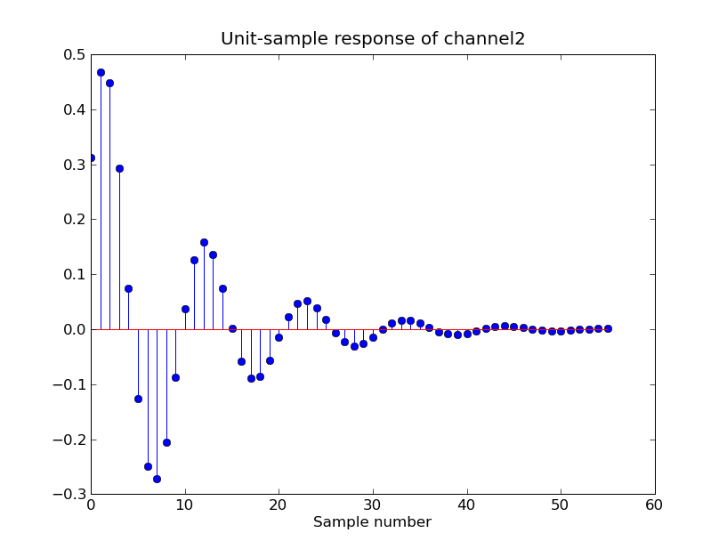
In lecture we saw that the unit-sample response completely characterizes the effect of a channel on sequences of samples that pass through the channel. So determining the response of a channel is a handy way to model a channel and (as we'll see in Task #6) is also useful in figuring out how to engineer the receiver to compensate for a channel's less desirable effects.
The unit-sample response is always measured by testing the channel with a single sample that has the value 1.0, followed by zero samples -- the digital signaling specification we're using doesn't play a role in this step. The Python expression [1.0]+[0.0]*k will build a (K+1)-sample sequence for testing the channel. If you call one of the channel functions with this test sequence as the argument, the sequence that is returned is the unit-sample response of the channel.
There's a small complication: officially the unit-sample response extends for an infinite number of samples. For all practical purposes it'll be very close to zero after a modest number of samples and our unit-sample response channel model will still be very accurate even if we truncate the response after it has effectively died out. Note that you'll need a unit-sample input sequence that's long enough to guarantee that you'll have sufficient response samples to find the right place to do the truncation.
Write a Python function unit_sample_response that returns a truncated sequence of samples that corresponds to the unit-sample response of the specified channel:
lab2_3.py is a template file for this task:
# template for Lab #2, Task #3
import numpy
import matplotlib.pyplot as p
import lab2

# turn on interactive mode, useful if we're using ipython
p.ion()

def unit_sample_response(channel):
    """
    Return sequence of samples that corresponds to the unit-sample
    response of the channel.  The sequence is truncated at the
    point where the absolute value of 10 consecutive samples is
    less than 1% of the value is the largest magnitude.
    """
    pass

if __name__ == '__main__':
    # plot the unit-sample response of our two channels
    lab2.plot_unit_sample_response(unit_sample_response,lab2.channel1)
    lab2.plot_unit_sample_response(unit_sample_response,lab2.channel2)

    # interact with plots before exiting.  p.show() returns
    # after all plot windows have been closed by the user.
    # Not needed if using ipython
    p.show()
The test code uses your function to compute the unit-sample response of our two channels and plots the result. If your function is working correctly you should see something like
Interview questions:
Task 4: Predicting channel behavior using the convolution sum (2 points)
We also saw in lecture that given the unit-sample response we can compute the effect of the channel on an arbitrary input by performing the appropriate convolution sum.
Write a Python script that does the following for each of the two channels mentioned in Task #2:
There is no template file for this task -- just organize the Python script as you think best and submit the result.
Interview questions:
Task 5: Generating eye diagrams (2 points)
Eye diagrams were introduced in lecture as a very effective way to visualize how a channel affects the sample sequences that pass through it. Recall that an eye diagram is just a plot of the channel output, but instead of stretching time out along the x axis of the plot, we make many overlayed plots of the output waveform, each overlay corresponding to the next short segment of time. The length of a plot segment is some small multiple of the time necessary to transmit one bit of the message.
Write a Python function plot_eye_diagram that generates a new figure containing an eye diagram for the channel function passed as an argument:
For this task, use the transmission of a random message sequence to provide data for your eye diagram. You can build the message by importing the random module and calling random.randint(0,1) repeatedly and collecting the results in a list. 200 message bits should do the trick.
In order to ensure one complete eye (typically covering the second half of one bit cell and the first half of the next) in the diagram, include enough plot samples to cover two bit cells (i.e., set plot_samples to 2*samples_per_bit.
Once your function is working, experiment with the value of samples_per_bit for both channels. Try to find the minimum value that produces an eye that's open enough to permit successful reception of the transmitted bits. You should find that the minimum value is different for the two channels.
lab2_5.py is a template file for this task:
# template for Lab #2, Task #5
import random
import matplotlib.pyplot as p
import lab2

# turn on interactive mode, useful if we're using ipython
p.ion()

def plot_eye_diagram(channel,samples_per_bit=8,plot_samples=16):
    """
    Plot eye diagram for given channel using a 200-bit random
    message.  samples_per_bit determines how many samples
    are sent for each message bit. plot_samples determines
    how many samples should be included in each plot overlay.
    plot_samples should be an integer multiple of samples_per_bit.
    """
    pass  # your function here

if __name__ == '__main__':
    # plot the eye diagram for both our channels

    # Experiment with different values of samples_per_bit for both
    # channels until you feel that the eye is open enough to permit
    # successful reception of the transmitted bits.  The result
    # will be different for the two channels.
    plot_eye_diagram(lab2.channel1,samples_per_bit=40)
    plot_eye_diagram(lab2.channel2,samples_per_bit=40)

    # interact with plots before exiting.  p.show() returns
    # after all plot windows have been closed by the user.
    # Not needed if using ipython
    p.show()
Interview questions:
Task 6: Deconvolution (3 points)
In lecture we talked about deconvolution, an approach to reconstructing the signal at the input to the transmission system by looking at the transmission channel's output (Y) and using the channel's unit-sample response (H).
In particular, we showed that the sequence W would be a reconstruction of the input sample sequence X if W satisfied the difference equation
y[n] = h[0]w[n] + h[1]w[n-1] + ... + h[K]w[n-K].
where Y is the sequence of channel output samples and the unit-sample response H is zero after some number of samples, i.e., h[n] = 0 when n > K.
We can rearrange this equation to solve for w[n]:
w[n] = (1/h[0])(y[n] - h[1]w[n-1] - ... - h[K]w[n-K]).
Since you are given Y, and since you know w[n] = 0 for n < 0, you can solve the above equation for w[0] given y[0], then for w[1] given w[0] and y[1], and so on:
w[0] = (1/h[0])(y[0])
w[1] = (1/h[0])(y[1] - h[1]w[0])
...
You will have to think carefully about how to modify this simple "plug and chug" strategy when the leading values of H (h[0], h[1],..) are zero.
lab2_6.py is a template for your Task 6:
# template for Lab #2, Task #6
import numpy,random
import matplotlib.pyplot as p
import lab2

def deconvolver(y,h):
    """
    Take the samples that are the output from a channel (y), and the
    channel's unit-sample response (h), deconvolve the samples, and
    return the reconstructed input.
    """
    pass  # your code here...

if __name__ == '__main__':
    """
    Develop test patterns and try using deconvolution to reconstruct
    the input from the output samples for each of the two channels.
    Use 8 samples per bit.  Generate plots comparing your
    reconstruction to the original input and output of the channel.
    Finally, try performing reconstruction with nonzero noise.
    """
    pass  # your code here...
There are three parts to this deconvolution task:
Note the unit-sample response of channel1 has leading zeros. Your code should handle this case correctly.
Interview questions: