Useful links
Numpy docs,
tutorial,
examples
Matplotlib.pyplot
reference,
tutorial
Goal
In this lab we'll look into what happens when a channel adds noise to the signal as it propagates from transmitter to receiver. We'll develop a mathematical model for noise, investigate how best to sample a noisy signal, and measure the number of bit errors caused by noise.
Instructions
See Lab #1 for a longer narrative about lab mechanics. The 1-sentence version:
Complete the tasks below, submit your task files on-line before the deadline, and complete your check-off interview within a week of the file submission deadline.
As always, help is available in 32-083 (see the Lab Hours web page).
Task 1: Computing sample statistics (2 points)
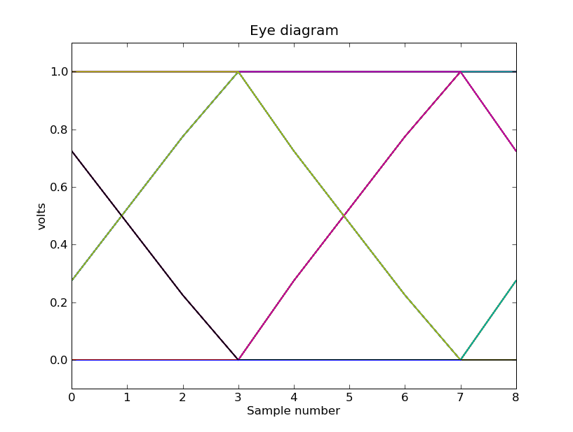
In Lab #2 we plotted eye diagrams for signals after they had passed through the channel. Here's an eye diagram generated by transmitting a random sequence of bits across an idealized channel that limits the speed of transitions and the inter-symbol interference extends only only to the next bit. The transmitter uses 4 samples/bit and signaling voltages of 0.0V and 1.0V.
If we choose a digitization threshold of 0.5V, we can see that in this noiseless world we could successfully sample this signal using any sample numbered 0 mod 4, 2 mod 4, or 3 mod 4 -- i.e., only if we tried to sample the signal at samples numbered 1 mod 4 would we make mistakes in determining which bit the transmitter intended to send. But to make the comparison with the digitization threshold as easy as possible, it would be best to choose the sample where the eye is most "open" -- samples numbered 3 mod 4 in this case.
As a first step in automating the process of determining where to sample, consider the following diagram which shows how the sample voltages are distributed at each of the four sample times within a bit cell. In the histogram for each of the four sample times, the length of the line indicates the fraction of samples that have the indicated voltage value.
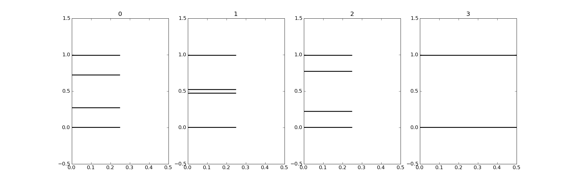
At sample times 0, 1 and 2 the samples are divided evenly among four possible intermediate voltages; at sample 3 the samples are divided evenly between the two final voltages 0.0V and 1.0V.
lab3_1.py is the template file for this task:
# this is the template for Lab #3, Task #1
import numpy
import lab3

def sample_stats(samples,samples_per_bit=4,vth=0.5):
    # reshape array into samples_per_bit columns by as many
    # rows as we need.  Each column represents one of the
    # sample times in a bit cell.
    bins = numpy.reshape(samples,(-1,samples_per_bit))

    # now compute statistics each column
    for i in xrange(samples_per_bit):
        column = bins[:,i]
        dist = column - vth
        min_dist = ???  # your code here
        avg_dist = ???  # your code here
        std_dist = ???  # your code here
        print "sample %d: min_dist=%6.3f, avg_dist=%6.3f, " \
              "std_dist=%6.3f" % (i,min_dist,avg_dist,std_dist)

if __name__ == '__main__':
    sample_stats(lab3.channel_data)
Finish the sample_statistics function given in the template so that for each of the four sample times within a bit cell it prints the following:
Interview questions:
Task 2: Modeling channel noise (3 points)
In lecture we learned that noise in transmission channels is actually the sum of a myriad of small perturbances, each of which has a value randomly chosen independently from a uniform distribution (where each value in the interval of possible values is equally likely to occur).
Let's run an experiment to get some idea of how noise values might be statistically distributed. Experiments using repeated random sampling are called Monte Carlo methods, named after the famous casino. Suppose that channel noise comes from 100,000 sources each of which contributes a voltage independently chosen from a uniform distribution in the range -0.001V to +0.001V. In a uniform distribution, all the probabilities are equal.
Some useful functions:
Write a Python function channel_noise that produces a noise value computed using the parameters above (100,000 sources, each contributing a value chosen from a uniform distribution in the range -0.001V to +0.001V).
Call channel_noise 10,000 times and produce a histogram of the results. You might want to start with, say, 100 calls to channel_noise until you are producing the histogram correctly. As we learned in lecture, we'd expect to find the results looking like a Gaussian distribution.
As it turns out (cf. Central Limit Theorem), we would get a Gaussian distribution for the total noise no matter what distribution we chose for the individual independent contributions as long as the distribution has a finite expected value and a finite variance.
Interview questions:
Task 3: Sampling in the presence of noise (1 point)
If we now add some noise to each channel (randomly chosen from the Gaussian distribution explored in Task #2) and plot the sample distribution, the figure from Task #1 now looks like
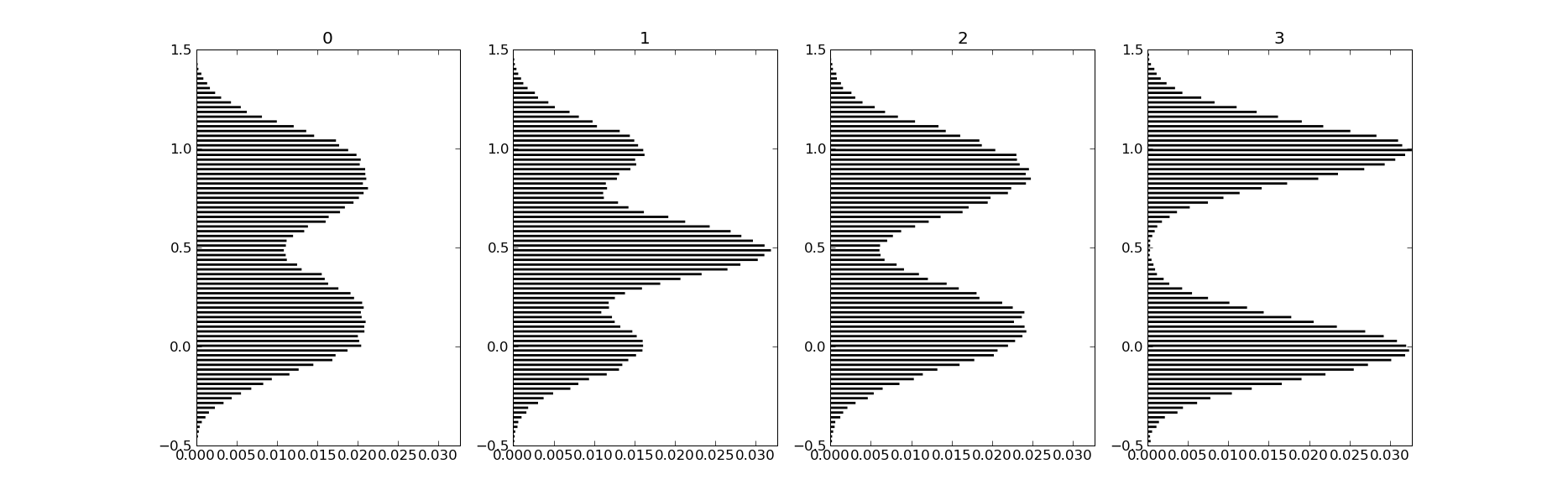
With noise, at each sample time we no longer see a sample distribution that only has samples at a small number of voltages -- each of the lines in the Task #1 histogram has been replaced by a Gaussian distribution centered where the lines used to be.
Rerun your code from Task #1, this time calling sample_stats with the argument lab3.noisy_channel_data. Think about the results and select the statistic you'll use to determine which sample number corresponds to the most open part of the eye.
Interview questions:
Task 4: Experimentally determining the bit error rate (2 points)
Using the results of your deliberations in Task #3, write a Python function receive that returns the recovered sequence of message bits given a vector of voltage samples produced by the channel:
Now write a second Python function bit_error_rate that compares to bit sequences and returns the fraction of bit locations that don't match. For example, if two 1000-element bit sequences mismatch in two bit locations, the result would be 2/1000 = .002.
# this is the template for Lab #3, Task #4
import matplotlib.pyplot as p
import math,numpy,random
import lab3

def receive(samples,samples_per_bit=4,vth=0.5):
    """
    Apply a statistical measure to samples to determine which
    sample in the bit cell should be used to determine the
    transmitted message bit.  vth is the digitization threshold.
    Return a sequence or array of received message bits.
    """
    pass # your code here

def bit_error_rate(seq1,seq2):
    """
    Perform a bit-by-bit comparison of two message sequences,
    returning the fraction of mismatches.
    """
    pass # your code here

if __name__ == '__main__':
    message = [random.randint(0,1) for i in xrange(1000000)]
    noisy_data = lab3.transmit(message,samples_per_bit=4,nmag=1.0)
    received_message = receive(noisy_data)
    ber = bit_error_rate(message,received_message)
    print "bit error rate = %g" % ber
Task 5: Computing the bit error rate (2 points)
Using some of the ideas from lecture we can derive an analytic estimate for the bit-error rate. In the experiments above we've been trying to determine the transmitted message bit by choosing samples from each bit cell where the eye was most open. In the idealized channel above, this turns out to sample time 3, the last of the four samples for each bit. Looking at the eye diagram from Task #1, we can see that at sample time 3 in the transmission of each bit, the expected sample voltage in a noise-free environment is 0.0V if we're transmitting a "0" bit and 1.0V if we're transmitting a "1" bit.
Now let's consider what happens when the channel adds noise to the signal. We'll get an error (i.e., receive a bit incorrectly) if there's sufficient noise so that the received sample falls on the wrong side of the threshold. For example, the transmission of a "1" would be received in error if
transmitted_voltage + noise_voltage ≤ threshold voltage
which is satisfied if the noise voltage &le -0.5V assuming we set the digitization threshold at 0.5V. Similarly, a transmitted "0" would be received in error if the noise voltage at that sample was ≥ 0.5V.
We can use these observations to develop a formula for the probability of a reception error at sample time 3 based on the probability of the noise voltage at that sample being larger or smaller than a certain amount:
p(error) = p(transmitted "1" received as "0") +
           p(transmitted "0" received as "1")

         = p(transmitted a "1") * p(noise ≤ -0.5) +
           p(transmitted a "0") * p(noise ≥ +0.5)

         = 0.5*p(noise ≤ -0.5) + 0.5*p(noise ≥ 0.5)
where we've used the information that we're transmitting a random bit stream so the probability of transmitting a "1" or a "0" is 1/2.
That just leaves figuring out the probabilities of the noise voltage being ≤ -0.5V or ≥ 0.5V. We've argued that the probability distribution function (PDF) for the noise is Gaussian, so the two probabilities we want are the shaded areas in the figure below.
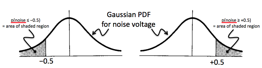
The area of the shaded regions can be determined from the cumulative distribution function (CDF) for the noise, defined for a value x as the integral of the PDF from -∞ to x, i.e., the probability that a value chosen according the PDF is ≤ x. So the area of the shaded area on the left is just the value of the CDF at -0.5, and, noting that the total area under the PDF is 1, the value of the shaded area on the right is 1 minus the value of the CDF at +0.5.
lab3.py includes the lab3.unit_normal_cdf(x) function which computes the value of the CDF at x for a unit normal PDF, i.e., a Gaussian PDF with a mean of 0 and a standard deviation of 1. The noise PDF used in this lab also has a mean of 0, but its standard deviation is 0.18, so we can't use lab3.unit_normal_cdf directly. But it's easy scale our argument (y) to one that can be used via the following formula:
x = (y - mean_of_y)/standard_deviation_of_y
Complete the calculation for p(error) using the formulas above and calls to lab3.unit_normal_cdf to come up with a numerical estimate for expected bit-error rate.
Interview questions: