Useful links
Goal
Write a decoder for convolutional codes based on the Viterbi algorithm. Measure the bit error rate for both hard-decision branch metrics and soft-decision branch metrics.
Instructions
See Lab #1 for a longer narrative about lab mechanics. The 1-sentence version:
Complete the tasks below, submit your task files on-line before the deadline, and complete your check-off interview within a week of the file submission deadline.
As always, help is available in 32-083 (see the Lab Hours web page).
Introduction
A convolutional encoder is characterized by two parameters: a constraint length k and a set of r generator functions {G0, G1, ...}. The encoder works through the message one bit at a time, generating a set of r parity bits {p0, p1, ...} by applying the generator functions to the current message bit, x[n], and k-1 of the previous message bits, x[n-1], x[n-2], ..., x[n-k-1]. The r parity bits are then transmitted and the encoder moves on to the next message bit. Since r parity bits are transmitted for each message bit, the code rate is 1/r.
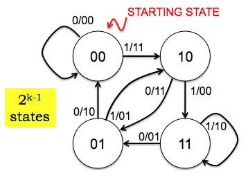
The operation of the encoder is best described as a state machine. The figure below is the state transition diagram for a rate 1/2 encoder with k=3 using the following two generator functions:
G0: 111, i.e., p0[n] = 1*x[n] + 1*x[n-1] + 1*x[n-2]
G1: 110, i.e., p1[n] = 1*x[n] + 1*x[n-1] + 0*x[n-2]
A generator function can described compactly by simply listing its k coefficients as a k-bit binary sequence, or even more compactly if we construe the k-bit sequence as an integer, e.g., G0: 7 and G1: 6.
In this diagram the states are labeled with the two previous message bits, x[n-1] and x[n-2], in left-to-right order. The arcs -- representing transitions between states as the encoder completes the processing of the current message bit -- are labeled with x[n]/p0p1.
You can read the transition diagram as follows: "If the encoder is currently in state 11 and if the current message bit is a 0, transmit the parity bits 01 and move to state 01 before processing the next message bit." And so on, for each combination of current states and message bits. The encoder starts in state 00.
The stream of parity bits arrives at the receiver; some of the bits may be received with errors because of noise introduced by the transmitter, channel and receiver. Based on the information in the (possibly corrupted) parity bits, the decoder deduces the sequence of states visited by the encoder and hence recovers the transmitted message. Because of errors, the receiver cannot know exactly what that sequence of states was, but it can determine the most-likely sequence using the Viterbi algorithm.
The Viterbi algorithm works by determining a path metric PM[s,n] for each state s and sample time n. Consider all possible encoder state sequences that leave the encoder in state s at time n. The most-likely state sequence is the one that transmitted the parity bit sequence that most closely matches the received parity bits, where the closeness of the match is determined by the Hamming distance between the transmitted and received parity bits: the smaller the Hamming distance, the closer the match. Each increment in Hamming distance corresponds to a bit error. The sequence with the smallest Hamming distance between the transmitted and received parity bits involves the fewest number of errors and hence is the most-likely (fewer errors being more probable than more errors). PM[s,n] records this smallest Hamming distance for each state at the specified time.
The Viterbi algorithm computes PM[…,n] incrementally. Initially
PM[s,0] = 0 if s == starting_state else ∞
The algorithm uses the first set of r parity bits to compute PM[…,1] from PM[…,0]. Then the next set of r parity bits is used to compute PM[…,2] from PM[…,1] and so on until all the received parity bits have been consumed.
Here's the algorithm for computing PM[…,n] from PM[…,n-1] using the next set of r parity bits to be processed:
For each state s:
Using the rate 1/2, k=3 encoder above, if s is 10 then, in no particular order, α = 00 and β = 01.
Continuing the example from step 1: p_α = 11 and p_β = 01.
Continuing the example from step 2: assuming the received parity bits p_received = 00, then BM_α = hamming(11,00) = 2 and BM_β = hamming(01,00) = 1.
PM_α = PM[α,n-1] + BM_α
PM_β = PM[β,n-1] + BM_β
PM_α is the Hamming distance between the transmitted and received parity bits so far assuming we arrive at state s via state α. Similarly, PM_β is the Hamming distance between the transmitted and received parity bits so far assuming we arrive at state s via state β.
Continuing the example from step 3: assuming PM[α,n-1]=5 and PM[β,n-1]=3, then PM_α=7 and PM_β=4.
if PM_α <= PM_β:
    PM[s,n] = PM_α
    Predecessor[s,n] = α
else
    PM[s,n] = PM_β
    Predecessor[s,n] = β
Completing the example from step 4: PM[s,n]=4 and Predecessor[s,n]=β.
We can use the following recipe at the receiver to determine the transmitted message:
Task 1: Implementing a Viterbi decoder? (6 points)
In this task we'll write the code for a Python class ViterbiDecoder. One can make an instance of the class, supplying k and the parity generator functions, and then use the instance to decode messages transmitted by the matching encoder.
The decoder will operate on a sequence of received voltage samples; the choice of which sample to digitize to determine the message bit has already been made, so there's one voltage sample for each bit. The transmitter has sent 0V for a "0" and 1V for a "1" but those nominal voltages have been corrupted by noise described by a Gaussian PDF with zero mean. 0's and 1's appear with equal probability in the original message, so the decoder should use a 0.5V threshold when digitizing the voltages into bits.
lab5_1.py is the template file for this task.
# This is the template file for Lab #5, Task #1
import numpy
import lab5

class ViterbiDecoder:
    # given the constraint length and a list of parity generator
    # functions, do the initial set up for the decoder.  The
    # following useful instance variables are created:
    #   self.k
    #   self.nstates
    #   self.r
    #   self.predecessor_states
    #   self.expected_parity
    def __init__(self,k,glist):
        self.k = k              # constraint length
        self.nstates = 2**(k-1) # number of states in state machine

        # number of parity bits transmitted for each message bit
        self.r = len(glist)

        # States are named using (k-1)-bit integers in the range 0 to
        # nstates-1. The bit representation of the integer corresponds
        # to state label in the transition diagram.  So state 10 is
        # named with the integer 2, state 00 is named with the
        # integer 0.

        # for each state s, figure out the two states in the diagram
        # that have transitions ending at state s.  Record these two
        # states as a two-element tuple.
        self.predecessor_states = \
          [((2*s+0) % self.nstates,(2*s+1) % self.nstates)
           for s in xrange(self.nstates)]

        # this is a 2D table implemented as a list of lists.
        # self.expected_parity[s1][s2] returns the r-bit sequence
        # of parity bits the encoder transmitted when make the
        # state transition from s1 to s2.
        self.expected_parity = \
          [[lab5.expected_parity(s1,s2,k,glist) \
            if s1 in self.predecessor_states[s2] else None
            for s2 in xrange(self.nstates)]
           for s1 in xrange(self.nstates)]

    # expected is an r-element list of the expected parity bits
    # (or you can also think of them as voltages given how we send
    # bits down the channel). received is an r-element list of
    # actual sampled voltages for the incoming parity bits.
    # This is a hard-decision branch metric, so, as described in
    # lab write up, digitize the received voltages to get bits and
    # then compute the Hamming distance between the expected sequence
    # and the received sequences, return that as the branch metric.
    # Consider using lab5.hamming(seq1,seq2) which computes the
    # Hamming distance between two binary sequences.
    def branch_metric(self,expected,received):
        pass  # your code here...

    # compute self.PM[...,n] from the batch of r parity bits and
    # the path metrics for self.PM[...,n-1] computed on the previous
    # iteration.  Follow the algorithm described in the lab
    # write up.  In addition to making an entry for self.PM[n,s] for
    # each state s, keep track of the most-likely predecessor
    # for each state in the self.Predecessor array.  You'll probably
    # find the following instance variables and methods useful:
    #    self.predecessor_states
    #    self.expected_parity
    #    self.branch_metric()
    def viterbi_step(self,n,received_voltages):
        pass  # your code here...

    # Identify the most-likely ending state of the encoder by
    # finding the state s which has the mimimum value of PM[s,n]
    # where n points to the last column of the trellis.  If there
    # are several states with the same minimum value, the end of
    # the message has been corrupted by errors, so decrement n
    # and repeat the search. Keep doing this until a unique s is
    # found.  Return the tuple (s,n).
    def most_likely_state(self,n):
        pass  # your code here...

    # starting at state s at time n, use the Predecessor
    # array to find all the states on the most-likely
    # path.  Each state contributes a message bit...
    def traceback(self,s,n):
        message = []
        while n > 0:
            # message bit that caused transition to
            # state s is also the high-order bit of
            # the state name
            message.append(s >> (self.k-2))
            # back to the next earlier state along the path
            s = self.Predecessor[s,n]
            n -= 1
        message.reverse()
        return message

    # figure out what the transmitter sent from info in the
    # received voltages
    def decode(self,received_voltages,debug=False):
        # figure out how many columns they'll be in the trellis
        nreceived = len(received_voltages)
        max_n = (nreceived/2) + 1

        # this is the path metric trellis itself, organized as a
        # 2D array: rows are the states, columns are the time points.
        # PM[s,n] is the metric for the most-likely path through the
        # trellis arriving at state s at time n.
        self.PM = numpy.zeros((self.nstates,max_n),dtype=numpy.float)

        # at time 0, the starting state is the most likely, the other
        # states are "infinitely" worse.
        self.PM[1:self.nstates,0] = 1000000

        # a 2D array: rows are the states, columns are the time
        # points, contents indicate the predecessor state for each
        # current state.
        self.Predecessor = numpy.zeros((self.nstates,max_n),
                                       dtype=numpy.int)

        # use the Viterbi algorithm to compute PM
        # incrementally from the received parity bits.
        n = 0
        for i in xrange(0,nreceived,self.r):
            n += 1

            # Fill in the next columns of PM, Predecessor based
            # on info in the next r incoming parity bits
            self.viterbi_step(n,received_voltages[i:i+self.r])

            # print out what was just added to the trellis state
            if debug:
                print self.PM[:,n],self.Predecessor[:,n]

        # find the most-likely ending state from the last row
        # of the trellis
        s,n = self.most_likely_state(n)

        # reconstruct message by tracing the most likely path
        # back through the matrix using self.Predecessor.
        return self.traceback(s,n)

    # print out final path metrics
    def dump_state(self):
        print self.PM[:,-1]

if __name__=='__main__':
    d = ViterbiDecoder(3,(7,6))
    received = numpy.array([1,1,1,0,1,1,0,0,0,1,1,0,0,0])
    message = d.decode(received,debug=True)
    print "decoded message =",message
The template contains a start at the implementation -- you'll get to finish the job! Here's a description of the functions you need to write:
Consider using lab5.hamming(seq1,seq2) which computes the Hamming distance between two binary sequences.
self.predecessor_states
self.expected_parity
self.branch_metric()
The testing code at the end of the template makes an instance of your decoder for the rate 1/2, k=3 code discussed in lecture. The received sequence is identical to the example used in Lecture #10, so the debugging printout showing the successive calculation of the path metrics and predecessor states should match what's shown on the slides.
Task 2: Error correction and BER (1 point)
In this task we'll run a simple experiment to measure the improvement in bit-error rate (BER) achieved by using a convolutional code. There's no code to write, just some results to analyze.
lab5_2.py is the template file for this task:
# This is the template file for Lab #5, Task #2
import lab5
from lab5_1 import ViterbiDecoder

if __name__=='__main__':
    # encode a 500,000 bit message using the specified
    # convolutional encoder, transmit it through a noisy
    # channel and then decode it with an instance of the
    # provided decoder class.  Compare the BER with simply
    # transmitting the raw message across the channel.
    lab5.test_ber(ViterbiDecoder,k=3,glist=(7,6),nbits=500000)

    # try it again with a stronger convolutional code
    lab5.test_ber(ViterbiDecoder,k=4,glist=(0xE,0xD),nbits=500000)
Run the code (be patient, it takes a while). If it's taking too long, try reducing nbits to 100000. Questions about the results:
Task 3: Soft-decision branch metrics (3 points)
Let's change the branch metric to use a "soft" decision based on the actually received voltages instead of just digitizing them directly to bits. As pointed out in lecture, there's a difference in likelihood between a "1" arriving as .999V and one arriving as .501V.
The soft metric we'll use is the square of the Euclidean distance between the received vector (of dimension r) of analog voltage samples and the expected r-bit vector of parities. Just treat them like a pair of r-dimensional vectors and use the usual formula for computing the square of the distance between the two vectors.
lab5_3.py is the template file for this task:
# This is the template file for Lab #5, Task #3
import lab5
from lab5_1 import ViterbiDecoder

class SoftViterbiDecoder(ViterbiDecoder):
    # override the default branch metric with one based
    # the square of the Euclidian distance between the
    # expected and received voltages.
    def branch_metric(self,expected,received):
        pass  # your code here...

if __name__=='__main__':
    # try both decoders on exactly the same noisy
    # received voltages
    lab5.test_two(ViterbiDecoder,SoftViterbiDecoder,
                  k=3,glist=(7,6),nbits=100000)
Complete the coding of the branch_metric method for the SoftViterbiDecoder class. Note that other than changing the branch metric calculation, the decoders are identical.
The test_two test function tests two decoders on exactly the same sequence of noisy received voltages. Since soft-decision Viterbi decoding is more effective than hard-decision decoding, we've increased the noise on the channel, so the results aren't directly comparable to those of Task #2.
Try running your code several times. What were the results of the bake-off? Should soft-decision decoders be preferred by better coders nationwide?