Overview

In this lab you'll do the following:

• Set up and read signals from an external microphone using the built-in Analog to Digital Converter that comes with most Series 7 Xilinx chips
• Build a voice recorder that records and plays back signed 8-bit digital audio samples.
• Implement a low-pass FIR filter module that can be used as an anti-aliasing and reconstruction filter.
• Implement one more optional element.
• Profit

Please be ready with the following when checking off for the audio lab:

• Have your Verilog code ready to be examined on the computer monitor.
• Demonstrate with Simulation/testbench of your FIR filter by displaying the 1khz and 5khz input and the filtered output. Explain why the peaks of the 1khz and 5khz input is out of phase with the filtered 1khz output.
• Demonstrate your recorder without the low-pass filter
• Demonstrate your recorder with the low-pass filter.

The Checkoff for this lab is worth 4 points for the functionality above and a full 5 points if you implement an echo effect (see the last section).

Please also be ready to answer the following questions:

• The low-pass filter is a simple example of digital signal processing (DSP). How can the FPGA be used to implement more sophisticated DSP functions, e.g., how would you add echo (reverb) to your playback audio signal?
• What is the longest recording sample you could have using all the BRAM on the Artix 7?

When you're done remember to upload your Verilog files to the course website so that they can be reviewed.

Files for this lab are found below:

• lab5_audio.sv, The main file which you'll be working in.
• nexs4ddr_audio.xdc (Use this one it is slightly modified than the general one).
• fir_31_tb.sv, a testbench for debugging your FIR filter.
• fir31.waveform, a two-sine wave input file for testing FIR filter.
• fir31.impulse, an impulse input file for testing FIR filter.

Audio Pipeline

We'll briefly go over the entire audio pipeline in this system so you'll have a general idea of how to fit things together. This section will also discuss creating instances of two IP modules (XADC Wizard and Block Memory Generator) that are used in this project, so please make sure to read through and do what it says!

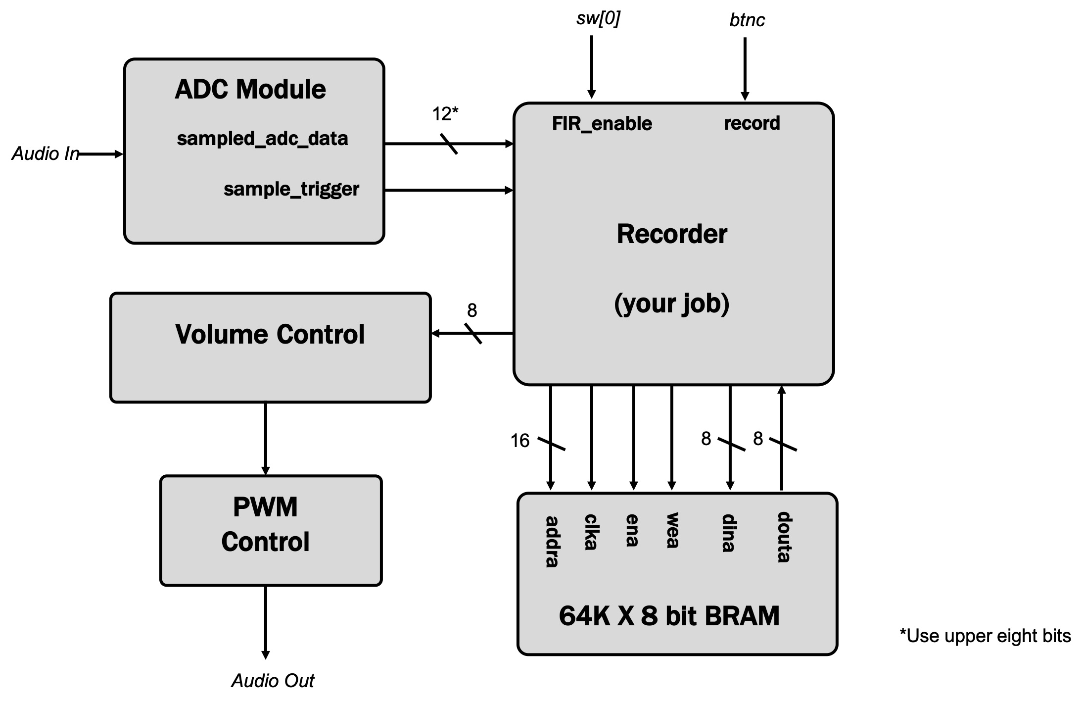
You'll be developing the recorder module which will interface with data coming from the Analog-to-Digital Converter, store data in and/or read data from from Block RAM (Random Access Memory), and then send an output signal to a PWM-audio generator.

Audio Generation

The audio generation portion of the project is already in place and can be demonstrated with the the lab5_audio.sv starter code. The starting form of the recorder module is comprised of two sine-wave generators which are selectively routed to the output (using a repurposed filter_in signal to choose between a 440Hz and 750Hz tone. Don't worry, filter_in will actually be used to specify a filter later, but for now we're just using it for another thing).

The sine_generator module generates sine waves based on the specified PHASE_INCR parameter. The sine generator represents \(2\pi\) of phase using an unsigned 32 bit number (and takes advantage of the fact that phase is \(\text{mod } 2\pi\) in the fact that a 32 bit number automatically wraps around as well).

module sine_generator ( input clk_in, input rst_in, //clock and reset
                        input step_in, //trigger a phase step (rate at which you run sine generator)
                        output logic [7:0] amp_out); //output phase   
    parameter PHASE_INCR = 32'b1000_0000_0000_0000_0000_0000_0000_0000>>5; //1/64th of 48 khz is 750 Hz
    logic [7:0] divider;
    logic [31:0] phase;
    logic [7:0] amp;
    assign amp_out = {~amp[7],amp[6:0]};
    sine_lut lut_1(.clk_in(clk_in), .phase_in(phase[31:26]), .amp_out(amp));
    
    always_ff @(posedge clk_in)begin
        if (rst_in)begin
            divider <= 8'b0;
            phase <= 32'b0;
        end else if (step_in)begin
            phase <= phase+PHASE_INCR;
        end
    end
endmodule

The top 6 bits of the phase generated is then used to “look up” a corresponding amplitude and that is ultimately sent out of module.

//6bit sine lookup, 8bit depth
module sine_lut(input[5:0] phase_in, input clk_in, output logic[7:0] amp_out);
  always_ff @(posedge clk_in)begin
    case(phase_in)
      6'd0: amp_out<=8'd128;
      6'd1: amp_out<=8'd140;
      6'd2: amp_out<=8'd152;
      //...
      //...
      6'd63: amp_out<=8'd115;
    endcase
  end
endmodule

To tune the sine generator's frequency, we specify the amount of normalized phase (\(0\) to \(2^{32}-1\) for \(0\) to \(2\pi\), respectively) to step on each step_in pulse, which in this lab is provided at 48 kHz. The module defaults to 750 Hz, which means PHASE_INCR starts at 1/64th of the sample rate of 48 kHz (which is why PHASE_INCR's default is specified that way). If one wanted a different frequency, such as 440Hz, the new phase increment step would be calculated as follows:

$$ \frac{\left(440\frac{\text{cycles}}{s}\right)\cdot \left(2\times 10^{32}-1 \frac{\text{phase}}{\text{cycle}}\right)}{48\times 10^{3}\frac{\text{samples}}{s}} \approx 39370534 \frac{\text{phase}}{\text{sample}} $$

You can see that number being used to instantiate the second instance of sine_generator below.

module recorder(
  input logic clk_in,              // 100MHz system clock
  input logic rst_in,               // 1 to reset to initial state
  input logic record_in,            // 0 for playback, 1 for record
  input logic ready_in,             // 1 when data is available
  input logic filter_in,            // 1 when using low-pass filter
  input logic signed [7:0] mic_in,         // 8-bit PCM data from mic
  output logic signed [7:0] data_out       // 8-bit PCM data to headphone
); 
    logic [7:0] tone_750;
    logic [7:0] tone_440;
    //generate a 750 Hz tone
    sine_generator  tone750hz (   .clk_in(clk_in), .rst_in(rst_in), 
                                 .step_in(ready_in), .amp_out(tone_750));
    //generate a 440 Hz tone
    sine_generator  #(.PHASE_INCR(32'd39370534)) tone440hz(.clk_in(clk_in), .rst_in(rst_in), 
                               .step_in(ready_in), .amp_out(tone_440));                          
    //logic [7:0] data_to_bram;
    //logic [7:0] data_from_bram;
    //logic [15:0] addr;
    //logic wea;
    //  blk_mem_gen_0(.addra(addr), .clka(clk_in), .dina(data_to_bram), .douta(data_from_bram), 
    //                .ena(1), .wea(bram_write));                                  
    always_ff @(posedge clk_in)begin
        data_out = filter_in?tone_440:tone_750; //send tone immediately to output
    end                            
endmodule 

The output of the recorder is fed into a volume_control module which scales (by factors of two) the amplitude of the signal it is provided. You can adjust the volume of the playback using sw[15:13]. When sw[15:13] is 3'b111, volume is maximized and when it is 3'b000 volume is minimized(but not zero, so don't be surprised if you still hear a tiny bit of sound).

Volume Control then sends its output to the PWM module which converts the signed 8 bits back to 8 bit offset binary, and then generates a PWM signal at 400 kHz used to drive the amplifier!

volume_control vc (.vol_in(sw[15:13]),
                   .signal_in(recorder_data), .signal_out(vol_out));
pwm (.clk_in(clk_100mhz), .rst_in(btnd), .level_in({~vol_out[7],vol_out[6:0]}), .pwm_out(pwm_val));
assign aud_pwm = pwm_val?1'bZ:1'b0; 

Build and test the starting form of lab5_audio.sv to make sure you are getting audio output.

Audio Input and the XADC Wizard

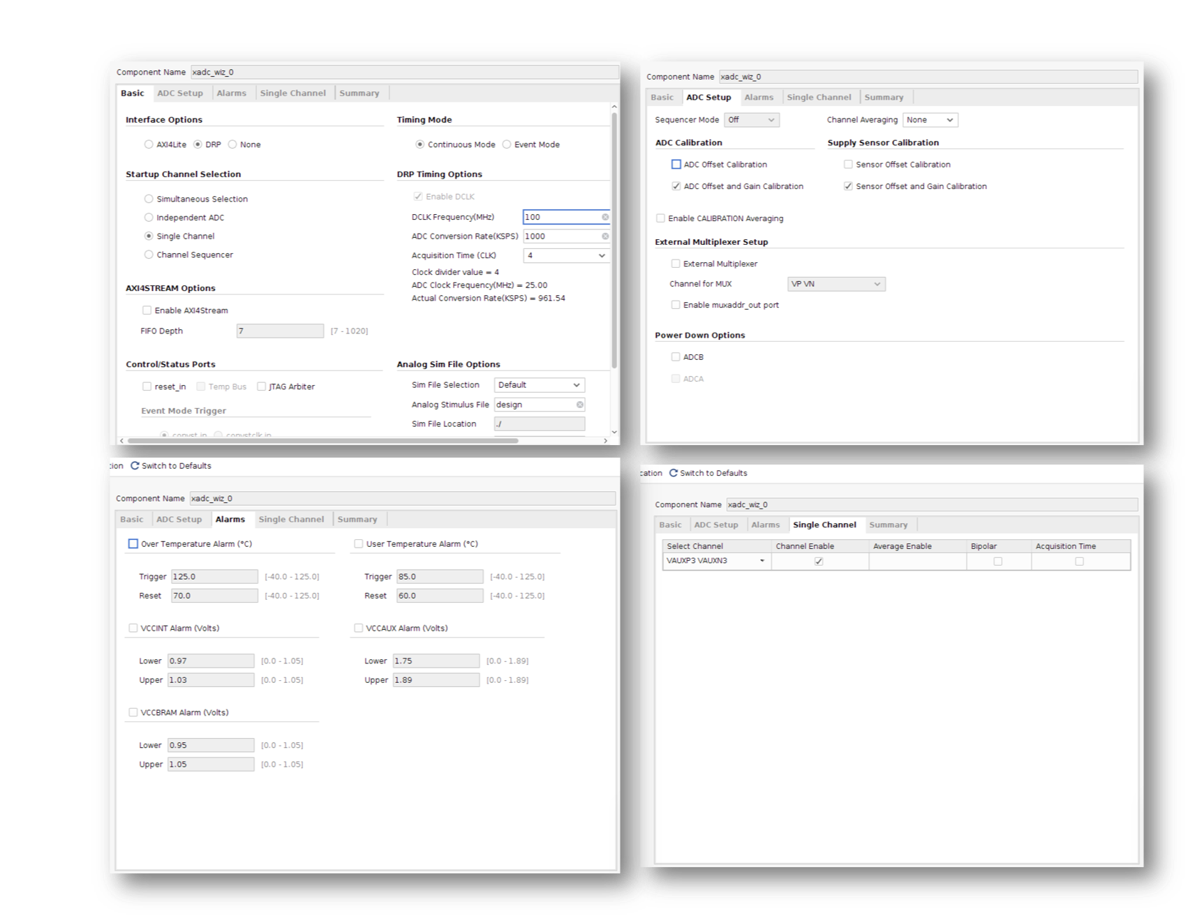
The Artix 7 FPGA on our Nexys 4 board is equipped with an input between the analog world and the primarily digital world of the FPGA. We use the XADC wizard in order to break out this functionality! You therefore need to create an instance of the XADC interfacer. The code to interface to it is already included (commented out) in the top_level module. Uncomment it, but in order for it to mean something, we need to add a new IP instance by searching for XADC under IP catalog. When the wizard comes up, make sure to select the following options:

• Under the Basic Tab make sure that things are set to:
  • DRP Mode (This sets up the ADC as a “Dynamic Reconfigurable Port”...basically this means that we're interfacing with the raw ADC and there's no additional logic being used...believe it or not this can make things easier!)
  • Single Channel
  • Continuous Mode
  • DCLK is 100 MHz
  • Uncheck the reset_in box.
• Under Alarms make sure all alarms are unchecked
• Under Single Channel pick: VAUX3P and VAUX3N in the first column: This specifies which external inputs are being sampled (AD3P and AD3N on the Nexsys board) make sure Channel Enable is checked.

Various settings used are shown for clarity below:

The “shape” of the module is also shown below for reference.

For future reference, the manual for the XADC is pretty good reading.

When done, click OK/Create and it'll generate it (like it has for other IP modules in the past).

The (previously-commented) code for interfacing with the xadc_interface you just made should minimize warnings about disconnected pins.

xadc_wiz_0 my_adc ( .dclk_in(clk_100mhz), .daddr_in(8'h13), //read from 0x13 for channel vaux3
                    .vauxn3(vauxn3),.vauxp3(vauxp3),
                    .vp_in(1),.vn_in(1),
                    .di_in(16'b0),
                    .do_out(adc_data),.drdy_out(adc_ready),
                    .den_in(1), .dwe_in(0));

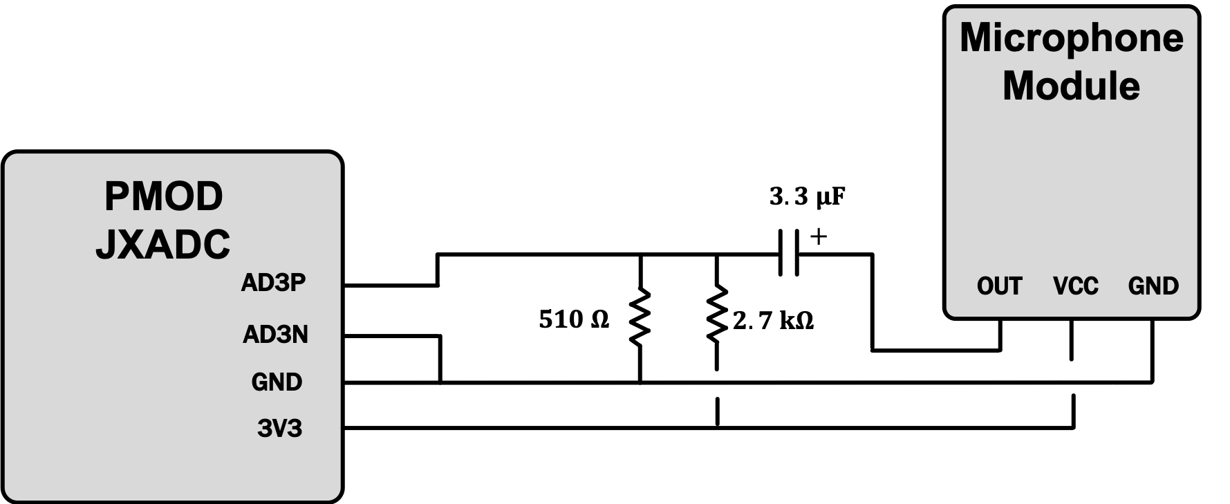
What you've just done is create an ADC interface to the AD3P and AD3N pins on the JXADC PMOD port (the upper right PMOD port on the board). This ADC will measure the voltage between the AD3P and AD3N pins. The maximum value this port can measure is +1V and minimum is 0V, using 12 bits to quantize the measurements (12'h000 is the lowest value and 12'hFFF is the highest. We'll attach a small microphone module to the ADC input channgel using a simple circuit shown below. Resistors, capacitors, microphones, breadboards, and wires should be available up front.

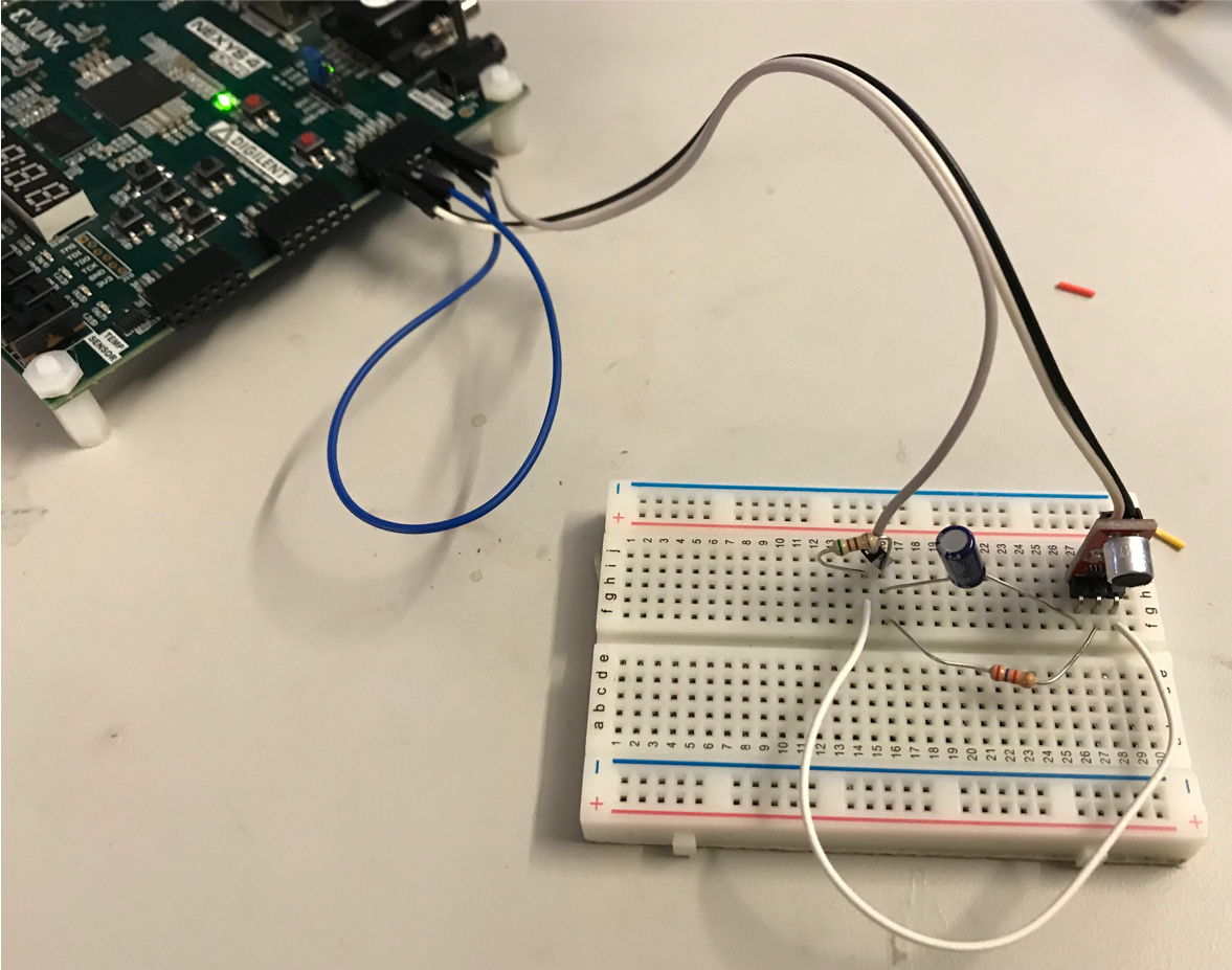
In real-life the setup looks like the following:

And also as a reminder, the PMOD connection has the following general pin format, with AD3P and AD3N being on pins 0 and 4, respectively.:

The ADC as set, will sample the microphone approximately 1 million times a second. We could have changed it so that its sample rate is much slower when setting up the ADC, but instead, we'll down-sample it to 48 kHz manually using a parameter called SAMPLE_COUNT in our verilog.

The audio signal coming in from the microphone varies from 0 to 1.0V with a 0.5 V offset (no sound therefore corresponds to about 0.5V). Consequently a “zero” reading is going to have a value of 12'b1000_0000_0000, while a maximum reading will be 12'b1111_1111_1111 and a minimum reading will be 12'b0000_0000_0000. Our entire audio pipeline deals with signed 2's complement numbers, however. A quick way to convert this singled-sided ADC signal, which is often termed “offset binary” to 2's complement is to invert the msb. Details and justification for this are provided here. This might take a few minutes to accept as a reasonable thing to do..

assign sample_trigger = (sample_counter == SAMPLE_COUNT);

always_ff @(posedge clk_100mhz)begin
    if (sample_counter == SAMPLE_COUNT)begin
        sample_counter <= 32'b0;
    end else begin
        sample_counter <= sample_counter + 32'b1;
    end
    if (sample_trigger)
        sampled_adc_data <= {~adc_data[11],adc_data[10:0]}; //convert from offset binary to 2's comp.
end

Implement Basic Recording Without Filtering

The goal of this lab is to implement a voice recorder . The top-level plan is pretty simple — when recording, store the stream of incoming samples in a memory, and when playing back, feed the stored data stream back.

There are (of course) some interesting details:

We'll use the FPGA's block RAMs (BRAMs) to build the memory for saved audio samples. A good size (i.e., one that fits in the FPGA we have) for the memory is 64K locations of 8 bits. To increase the recoding time, let's down-sample the 48kHz incoming data to 6kHz, i.e., only store every eighth sample.

Modify the recorder module to implement basic record and playback functionality. You can build your 64Kx8 memory using Vivado's Block Memory Generator. Go to IP Catalog>Block Memory Generator, and generate a BRAM with the options highlighted below.

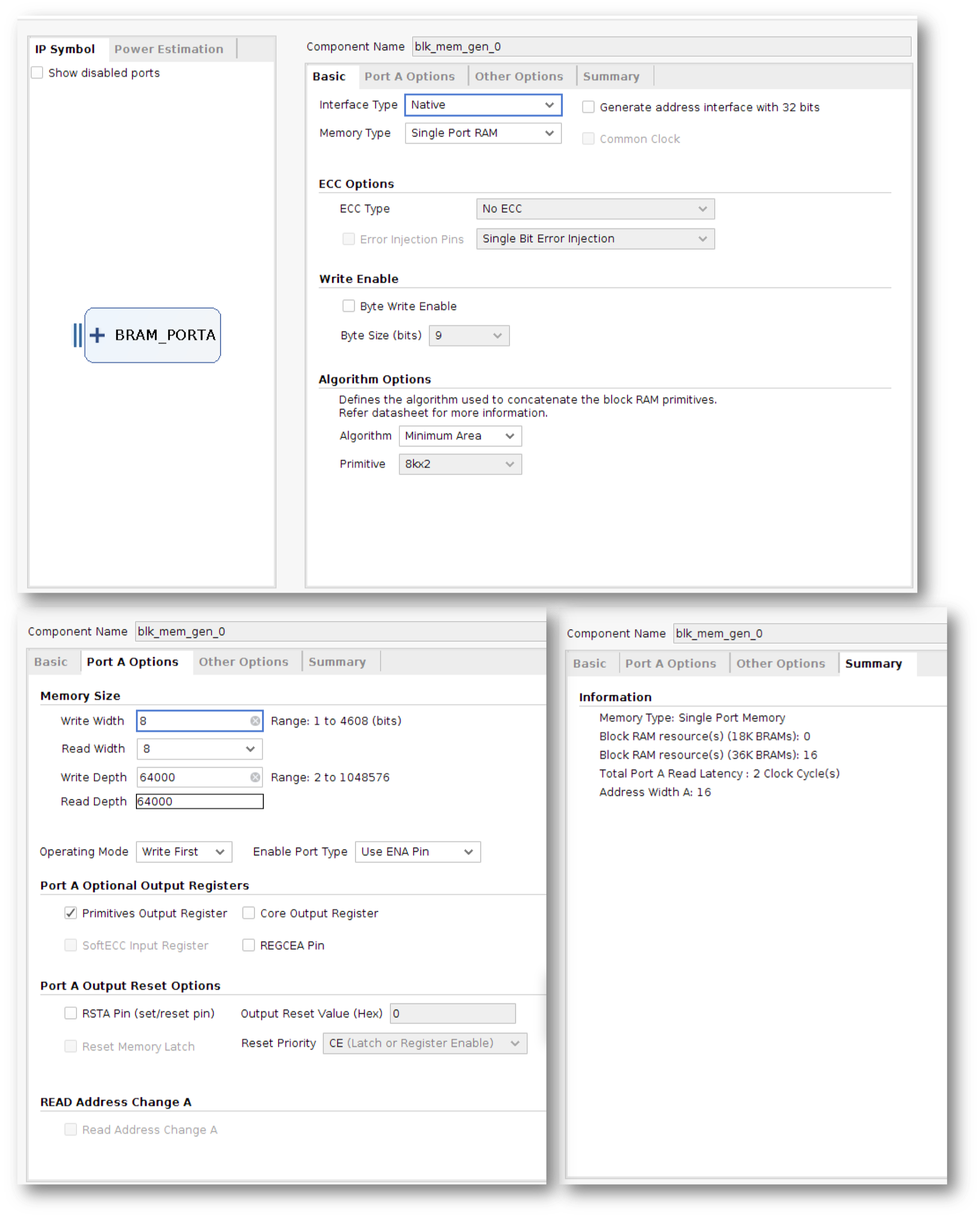
Once it has been created, uncomment the associated lines in the recorder module to create an instance of the BRAM IP you just generated.

blk_mem_gen_0 mybram(.addra(addr), .clka(clk_in), 
              .dina(data_to_bram), 
              .douta(data_from_bram), 
              .ena(1), .wea(write));        

The `recorder module has the following inputs and outputs:

• clk_in: system clock
• rst_in: 1 to reset the module to its initial state
• record_in: 1 for record, 0 for playback (connected to btnc in top_level)
• filter_in: 1 for filtering, 0 for no filtering (we'll ignore this part until the filter section). Connected to sw[0] in top_level.
• ready_in: transitions from 0 to 1 when a new sample is available
• mic_in [7:0]: 8-bit data from the microphone (signed, two's complement)
• data_out [7:0]: 8-bit signed data to the volume, and PWM module for output (signed, two's complement)

Your job now is to implement the record/playback module. There are two “modes” described below:

• Record Mode: When entering record mode, reset the memory address. When the ready_in input is asserted, a new sample from the microphone is available on the mic_in[7:0] input at the rising edge of clk_in. Store every eighth sample in the memory, incrementing the memory address after each write. You should also keep track of the highest memory address that's written. If you fill up memory, you should stop recording new samples.

• Playback Mode: When entering playback mode, reset the memory address you're reading from. When the ready_in input is asserted, supply a 8-bit sample on the data_out[7:0] output and hold it there until the next sample is requested. For now, read a new sample from the memory every eight transitions of ready and send it to the data_out eight times in a row (i.e., up-sample the 6kHz samples to 48kHz using simple replication). When you reach the last stored sample (compare the memory address to the highest memory address written which you saved in record mode), reset the address to 0 and continue — this will loop through the saved data again and again.

Low Pass Filter

Remembering about Nyquist rates, the original 48kHz data can represent audio frequencies up to 24kHz. Down-sampling to 6kHz yields data that can represent audio frequencies up to 3kHz. In order to prevent aliasing during the down-sampling process we'll need to remove audio frequencies between 3kHz and 24kHz from the data before down-sampling by passing the incoming samples through a low-pass anti-aliasing filter.

The outgoing data stream wants samples every 48kHz , which we currently produce by replicating each stored 6kHz sample eight times. But if we do that we will hear 6kHz noise (and its overtones) introduced by by the replication process. So we'll pass the outgoing samples through a low-pass reconstruction filter to ensure that the 48kHz output stream only contains audio frequencies up to 3kHz.

In fact we can use the same low-pass filter as both an anti-aliasing filter during recording and a reconstruction filter during playback. In order to implement our filter we'll be working with the following modules:

fir31 : The module that you'll be writing. It will act as a 31 tap Finite Impulse Response Filter (FIR Filter).

coeffs31: a combinational module that returns a signed 10-bit filter coefficient given a tap number between 0 and 30. The coefficients were determined by using the fir1(30,.125) command in Matlab, then scaling the result by 2**10 to produce integer tap coefficients. This module is already written and is available for your use.

Since we got recording working in the previous section, let's replace the simple pass-through code of the fir31 module with code that actually implements a 31-tap low-pass filter. The filter calculation requires forming the following sum:

$$ y[n] = \sum_{i=0}^{30}(c_i\cdot x[n-i]) $$

which in pseudo-code looks like:

y = sum(i from 0 to 30 (coeff[i] * sample[i]))

where coeff[i] is supplied by the coeffs31 module and sample[i] is reaching into a buffer of recent samples. sample[0] is the current sample, sample[1] is the previous sample, sample[2] is the sample before that, etc. We are in essence performing a convolution of the incoming audio signal with the values of our lowpass filter.

This would be a lot of multiplies and adds if we tried to do the calculation all at once — way too much hardware! Since our system clock (100MHz) is much faster than rate at which new samples arrive (48kHz) we have plenty of clock cycles to perform the necessary calculations over 31 cycles, using an accumulator to save the partial sum after each iteration.

Usually filter coefficients are real numbers in the range [−1,1] but realistically (for this lab anyway) we can only build hardware to do integer arithmetic. So the coefficients have been scaled by 2*10 (i.e., multiplied by 1024) and rounded to integers. That means our result is also scaled by 2*10, so instead of the output y being the same magnitude as the input samples, 8 bits, it's 18 bits. So the accumulator should be 18 bits wide.

Conceptually, the 31-location sample memory shifts with every incoming sample to make room for the new data at sample[0]. But this sort of data shuffling would be tedious to implement, energy inefficient, and resource inefficient so instead let's use a circular buffer. That's a regular memory with an offset pointer that indicates where index 0 is located. Use BRAM for large memory requirements and registers for small arrays. For the sample memory, it's easier to create the circular buffer with an array of registers:

logic [7:0] sample [31:0];  // 32 element array each 8 bits wide
logic [4:0] offset; //pointer for the array! (5 bits because 32 elements in above array! Do not make larger)

When we get a new sample, we increment the offset and store the incoming data at the location it points to in the array. Then sample[offset] is the current sample, sample[offset-1] is the previous sample, sample[offset-2] is the sample before that, etc. If we choose the sample memory size to be a power of 2 and make sure offset is the same size, then we don't have to worry about our pointer incrementing off into a no-no region like you do in the C programming language since the index arithmetic modulo is done automatically (overflowing is not always bad and can be a force for good) and the memory size and everything will work out correctly. (Note that the index for sample must be a 5 bit wire.) So now the formula becomes (in pseudo-code):

y = sum(i from 0 to 30 (coeff[i] * sample[offset-i]))

When we fit this math into the context of the module we need to build, here's specifically what it needs to do:

When ready_in is asserted, increment the offset and store the incoming data at sample[offset]. Set both the accumulator and index to 0. Over the next 31 system clock cycles (@ 100MHz) compute coeff[index] * sample[offset-index], add the result to the accumulator, and increment the index. Remember to declare coeff and the sample memory as signed so that the multiply operation is performed correctly (this is important!!). When index reaches 31, it's done and the accumulator contains the desired filter output! Now the module just waits until ready is asserted again and starts over.

With this implementation the filter looks like a one sample delay and can be easily spliced into the recording pipeline.

To help you test your fir31 module, we've written a Verilog test jig, fir31_test.v, which you can use with Behavioral Simulation to run your module through it's paces. When executed, the test jig reads the file fir31.samples (which you need to set to either fir31.impulse or fir31.waveform, feeds them to your module, captures the output value and writes it to the fir31.output file (if needed). There are two sample files:

• fir31.impulse which has a string of 0 samples, followed by a single sample of 1, followed by more 0 samples. The expected output should be 0's, followed by the coeffients of the 31 filter taps in order, followed by more 0s. (Remember a FIR filter is actually just convolution with a specific impulse response, so convolving with an impulse response should result in the taps of the FIR filter).
• The file fir31.waveform which has 48,000 samples of a waveform constructed by adding together 1kHz and 5kHz sine waves. The expected outputs are given in fir31.filtered, which is approximately a 1kHz sine waveform. The frequency plots of fir31.waveform and fir31.filtered are shown below — note how the 5kHz component has been filtered out!

Download fir31.impulse and/or fir31.waveform and rename the file name fir31.samples to point to where on your file system you placed the input file you want to test (either fir31.impulse and/or fir31.waveform).

The simulation will stop after the last input sample has been processed. Use the waveform viewer from the behavioral simulation to

Viewing the output of the FIR filter in the time domain provides a more intutitive picture. Input fir31.waveform (which has a 1khz and 5khz sinewave) as fir31.sample for your filter. Run the simulation for 20ms. Under properties in the waveform window, select Analog waveform (interpolated). You should see the a 1khz wave with a 5khz signal as the input. The filtered result shows a 1khz waveform with almost all of the 5khz signal removed as shown below

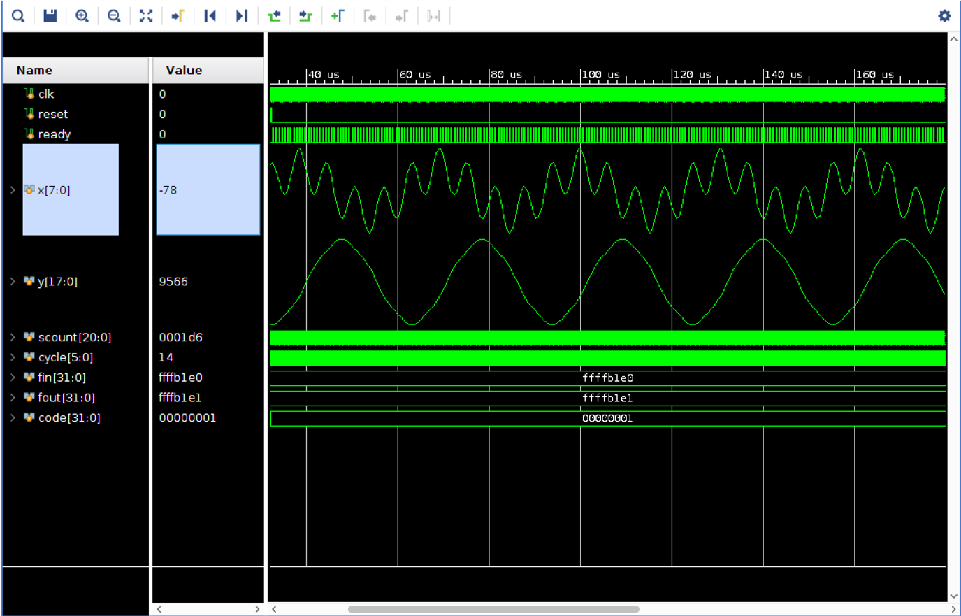
If this doesn't work, make your input file fir31.impulse and analyze the output that is generated. In response to an unit impulse the system should output all 31 tap values. Use this as a first step to debugging.

#Add In the Low-Pass Filter!

Once your filter is working, integrate a single instance of the fir31 module to your recorder module. Use muxes to route data to the filter inputs, memory inputs, and data_out signals as described below.

The previously ignored filter_in input to your recorder module (controlled by sw[0]) should now be used. When filter is 0, your recorder module should behave as before. When the filter switch is 1 the fir31 module should be used as an anti-aliasing filter during recording and as a reconstruction filter during playback.

Here's a table showing the connections during various modes of operation:

When the fir31 module is used as a reconstruction filter, it's input is a zero-expanded set of samples from the recording memory. “Zero expansion” is a type of up-sampling where one data sample is used from memory, followed by in our case seven samples of 0. The filter will interpolate between the memory samples, smoothly filling in values in place of the zeros. In this mode, the filter has a gain of 1/8 which we can compensate for by multiplying its output by 8. This is accomplished by simpling moving 3 bits to the right when selecting which output bits to use.

Try making both filtered and unfiltered recordings, and listen to both, with and without the filter enabled on playback. Without using the filter the playback will have some static (high-frequency noise) and, if you have young ears, you'll here high frequency tones that weren't in the original voice. Using the filter should suppress most of the audio artifacts.

If your recording without the FIR filter works perfectly but are having problems with the FIR filter, then it's mostly an implementation error in the FIR filter. It's not uncommon to have a buggy FIR filter yet show a perfect simulation!

Which filtering operation seems to have the biggest effect: anti-aliasing or reconstruction? During checkoff, show how the playback data changes when you switch the filter on and off.

Final Section Final Section Final Section (Echo)

For full-credit on this lab, you need to implement an Echo effect.

Echo

Add echo (reverb) to the playback audio signal. In audio signal processing, echo is a reflection of sound that arrives at the ear with a delay. The level is of course attenuated. There are two primary ways to implement an echo. The first is with some type of module that accesses values from the BRAM with an offset and adds them together. For example having three BRAM pointers is a possibility. This is most likely the easier way to go about this task for this lab.

The second, and generally more extensible approach, is to convolve your audio signal with the impulse response of an ideal echo. You could easily do this by creating a second FIR filter module and FIR coefficients module that will convolve your incoming audio with an echo signal. If you've done 6.003 before, you should have seen something like this before, but if not feel free to ask about it on Piazza! The FIR taps are really just the values that would result when an impules of noise is injected into a system. In the case of a FIR filter something like the following would be the FIR of a an echo-like system (although you'd probably want to implement it using signed whole numbers like we did in our FIR filter in this lab):

$$ [1,0,0,0,0.75,0,0,0,0.5,0,0,0,0.25] $$

This is an extremely powerful approach since basically anything (the acoustics of any room, for example), can be captured by using its impulse response as FIR taps, which then let's you do stuff like make your regular audio sound like it is coming from a stadium by convolving it with the impulse response of a stadium (and these impulse responses can be found online and elsewhere). It is pretty cool, if you ask us. If you choose to do it this way, you will want to use a BRAM to remember past values (and also realize that at 48 ksps, an echo-like FIR will have stretches of taps that are zero that are 1000's long)