Proof of Kelvin's Theorem (From JNN, page 103).

The circulation $\Gamma$ is defined as the integrated tangential velocity around any closed contour C in the fluid,

$$\Gamma = \int_{C}\vec{v}\cdot d\vec{x} = \int_{C}v_{i}dx_{i}.$$ (1)

Kelvin's theorem of the conservation of circulation states that for an ideal fluid acted upon by conservative forces (e.g., gravity) the circulation is constant about any closed material contour moving with the fluid. Physicaly, this happens because no shear stresses act within the fluid; hence it is impossible to change the rotation rate of the fluid particles. Thus, any motion that started from a state of rest at some initial time, will remain irrotational for all subsequent times, and the circulation about any material contour will vanish.

To proof Kelvin's theorem, we consider the derivative of (1) with respect to time $d\Gamma/dt$. Since the contour C moves with the fluid particles, or with velocity $\vec{v}$, it follows that

$$\frac{d\Gamma}{dt} = \frac{d}{dt}\int_{C}\vec{v}\cdot d\vec{x... ...al t}+v_{j}\frac{\partial}{\partial x_{j}}\right)(v_{i}dx_{i})$$ (2)

Here the differential operator acting upon the integrand is the substantial (material) derivative $D\Gamma/Dt$, since the contour of integration C is a material contour moving with the fluids particles. The resulting derivatives of the velocity components v_i are straightforward to compute, but some care is required for the differential element dx_i. Since C is a material contour, the differential element will itself be a function of time; to analyze its resulting distortion, we resort to the definition of the integral as the limit of a finite sum.

figure

 

Figure 1: Discrete representation of the material contour C.

Thus , if x_i⁽ⁿ⁾ denotes the coordinates of the nth point along the contour C, say with $n = 1,2,\ldots, N$, the integral in equation (2) can be replaced by the

$$\frac{d\Gamma}{dt} = \lim_{N \rightarrow \infty} \sum_{n}\lef... ...frac{\partial}{\partial x_{j}}\right)(v_{i}\delta x_{i}^{(n)})$$ (3)

provided that as $N \rightarrow \infty$,

$$\delta x_{i}^{(n)} \equiv x_{i}^{(n+1)}-x_{i}^{(n)} \rightarrow 0.$$ (4)

Since the coordinates x_i⁽ⁿ⁾ move with individual fluid particles, they must be functions of time. By definition the velocity components at the same points are given by

$$v_{i}^{(n)} = \frac{\partial x_{i}^{(n)}}{\partial t}.$$ (5)

Using the chain rule in equation (3), noting that the coordinates x_i⁽ⁿ⁾ depend on time but not on the space coordinates, and finally using equation (5), we obtain

$$\frac{d\Gamma}{dt} = \lim_{N \rightarrow \infty} \sum_{n}\lef... ...^{(n+1)}-x_{i}^{(n)})+v_{i}(v_{i}^{(n+1)}-v_{i}^{(n)})\right].$$ (6)

In this form, the limit is given by the integrals

$$\frac{d\Gamma}{dt} = \int_{C}\left(\frac{\partial}{\partial t... ...}{\partial x_{j}}\right)dx_{i}+\frac{1}{2}\int_{C}v_{i}dv_{i}.$$ (7)

Now, the first part of the integrand in (7) is the left hand side of Euler's equation. then we can rewrite equation (7) in the form

$$\frac{d\Gamma}{dt} = \int_{C}\frac{\partial}{\partial x_{i}}\... ...(p+\rho g x_{2}\right)dx_{i}+\frac{1}{2}\int_{C}d(v_{i}v_{i}).$$ (8)

The right side of equation (8) is the integral of a perfect differential over a closed contour and is, therefore, equal to zero. In effect, the integral can be integrated to give

$$-\frac{1}{\rho}\left[p+\rho g x_{2}-\frac{1}{2}\rho v_{j}v_{j}\right]_{A}^{B},$$

where A and B are the upper and lower limits of integration; since these points are identical, the difference $[\ldots]_{A}^{B} = 0$.

A Different Approach to Obtain $d\Gamma/dt$.

To proof Kelvin's theorem, we need to evaluate $d\Gamma/dt$, and in the proof above the representation of the integral as the limit of a finite sum was used to obtain the expression for $d\Gamma/dt$. Here we discuss how to obtain this expression using the definition of the derivative. We write

$$\frac{d\Gamma}{dt} = \lim_{\Delta t \rightarrow 0}\frac{\int_... ...x} -\int_{C(t)}\vec{v}(t,\vec{x}(t))\cdot d\vec{x}}{\Delta t}.$$ (9)

For a fluid particle at position $\vec{x}(t+\Delta t)$ (a point over the material contour $C(t+\Delta t)$), we can write in the limit $\Delta t \rightarrow 0$ that

$$\vec{x}(t+\Delta t) \approx \vec{x}(t)+\frac{d \vec{x}}{d t}(t)\Delta t + O((\Delta t)^{2}).$$ (10)

The speed $\vec{v}$ of a fluid particle at the position $\vec{x}$ is given by the equation

$$\frac{d\vec{x}}{dt}(t) = \vec{v}(t,\vec{x}(t)).$$ (11)

Therefore, equation (10) can be written in the form

$$\vec{x}(t+\Delta t) \approx \vec{x}(t)+\vec{v}(t,\vec{x}(t))\Delta t + O((\Delta t)^{2}).$$ (12)

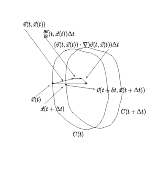
This equation is illustrated in the figure below. In the limit $\Delta t \rightarrow 0$, the position $\vec{x}(t+\Delta t)$ (a point of the material contour $C(t+\Delta t)$) of a fluid particle at the instant $t+\Delta t$ can be approximated by its position $\vec{x}(t)$ (a point over the material contour C(t)) at instant t, plus what it has traveled during the time $\Delta t$. The distance traveled is given approximately by the vector $\vec{v}(t,\vec{x}(t))\Delta t$ with an error of order $O((\Delta t)^{2})$.

figure

 

Figure: Contours C(t) and $C(t+\Delta t)$. Illustration of the approximation for $\vec{x}(t+\Delta t)$.

According to equation (12), we can write

$$d\vec{x}(t+\Delta t) \approx d\vec{x}(t)+d\vec{v}(t,\vec{x}(t))\Delta t + O((\Delta t)^{2}).$$ (13)

The velocity vector $\vec{v}$ at the instant $t+\Delta t$ can be approximated in the same way as $\vec{x}(t+\Delta t)$ and $d\vec{x}(t+\Delta t)$. We can write

$$\vec{v}(t+\Delta t,\vec{x}(t+\Delta t)) \approx \vec{v}(t,\ve... ...{\partial t}(t,\vec{x}(t+\Delta t))\Delta t+O((\Delta t)^{2}).$$ (14)

If we substitute the approximate expression for $\vec{x}(t+\Delta t)$, given by equation (12), into equation (14), we obtain

$$\vec{v}(t+\Delta t,\vec{x}(t+\Delta t)) \approx \vec{v}(t,\ve... ...}(t)+\vec{v}(t,\vec{x}(t))\Delta t)\Delta t+O((\Delta t)^{2}).$$ (15)

Now we expand $\vec{v}$ in taylor series with respect to the second variable to obtain

$$\vec{v}(t+\Delta t,\vec{x}(t+\Delta t)) \approx \vec{v}(t,\ve... ...}\cdot\nabla \vec{v}(t,\vec{x}(t))\Delta t+ O((\Delta t)^{2}).$$ (16)

The expanssion above is illustrated in the figure below

According to equations (13) and (16), the integrand of the first integral in the right hand side of equation (9) can be approximated by the equation

$$\begin{split} \vec{v}(t+\Delta t,\vec{x}(t+\Delta t))\cdot d\... ...t d\vec{v}(t,\vec{x}(t))\Delta t+O((\Delta t)^{2}). \end{split}$$ (17)

Notice that the approximated form of the integrand of the first integral in the right hand side of equation (9), given above by equation (17), is now being evaluated over the contour C(t) instead of the contour $C(t+\Delta t)$. Therefore, we can write

$$\begin{split} \int_{C(t+\Delta t)}\vec{v}(t+\Delta t,\vec{x}(... ...c{v}(t,\vec{x}(t))\Delta t \\ & +O((\Delta t)^{2}). \end{split}$$ (18)

Now we can replace the first integral in the right hand side of equation (9) by the expression given in the equation (18). Therefore, the time derivative of the circulation is

$$\frac{d\Gamma}{dt} = \lim_{\Delta t \rightarrow 0}\left\{\int... ...t,\vec{x}(t))\cdot d\vec{v}(t,\vec{x}(t))+O(\Delta t)\right\},$$ (19)

and after the limit process is taking into account, we obtain

$$\frac{d\Gamma}{dt} = \int_{C(t)}\left(\frac{\partial \vec{v}}... ...+\int_{C(t)}\vec{v}(t,\vec{x}(t))\cdot d\vec{v}(t,\vec{x}(t)),$$ (20)

which is exactly the equation (7) we obtained using the previous approach.