Contents
- 1 Introduction
- 2 Desired Kinematics
- 3 Concept generation
- 3.1 Using an old solution
- 3.2 Constraint-Based Design
- 3.3 Topological Synthesis
- 3.4 FACT
- 3.5 Transmission Theory
- 4 Range of Motion
- 5 Stiffness
- 6 Load Capacity
- 7 Dynamics
- 8 Fatigue
- 9 Repeatability
- 10 Error Budget
- 11 Optimization
- 12 Fabrication
1 Introduction
Flexures are bearings that allow motion by bending load elements such as beams. The arrangment of beams can be designed to be compliant in its degree(s) of freedom (DOF), but relatively stiff in its degree(s) of constraint (DOC). This allows engineers to provide motion in desired directions, but constraint in other directions. Flexures are important for engineers because they allow stiction-less, controlled, limited-range motion. These well-designed, well-understood springs can then be implemented in precision machines to allow the development of medical devices and machines for electronic fabrication. This entry is about understanding the most important parameters for flexure design. The functional requirements for flexures include (but are not limited to): desired kinematics, range of motion, stiffness, load capacity, repeatability, mode shapes/frequencies, and an error budget.
Designing flexures involves developing a model, using FEA, and experimentally verifying the models. There should be a pencil-and-paper approximation that allows you to see which variables are most important and it gets you in the ballpark of the correct dimensions. In other words, the model shows you which direction to go and by how much. How short can I make this beam so that it can be at 30% of the yield stress? The model should answer questions like that, keeping real-world constraints in mind.
By carefully applying these equations to your system, you should have a decent approximation for its behavior. Once the equations are developed, you should put these variables in a MATLAB script or an Excel spreadsheet. That way, you can change one variable at a time and see how that affects the entire system. Flexures are typically modeled using FEA, which is the subject of another entry.
2 Desired Kinematics
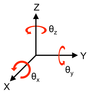 The first step in flexure design is to identify the degrees of freedom. These are the desired directions of travel. Conversely, you could find the desired constraints first. That is, it may be easiest to identify which directions are undesirable for travel. Every rigid body has six degrees of freedom: three for translation and three for rotation. Keep in mind that the flexures that you design will not be infinitely stiff in the constraint directions, but if designed properly will be orders of magnitude stiffer than the degrees of freedom.
Once the degrees of freedom are identified, they should be characterized. That is, the required ranges of motion in the degrees of freedom and constraint should be specified. These specifications will aid the choice in flexure topology.
3 Concept Generation
Flexure concepts can be generated once the kinematics have been identified. There are several methods, including using an old solution, constraint-based design, topological synthesis, Freedom, Actuation, and Constraint Topologies (FACT), and Transmission Theory (a major contribution from my Master's thesis.) FACT is an intuitive and powerful tool for flexure design. See chapter 1 of my Master's thesis for more information on these techniques.
3.1 Using an old solution
There have been several flexure designs that have been developed already. There is a nice list in the back of the book "The Handbook of Compliant Mechanisms." Also, there is a way to transform linkages into flexures: the pseudo-rigid body model (PRBM) developed by Larry Howell.
3.2 Constraint-Based Design
Constraint-based design generates compliant mechanisms via flexural building blocks. An example of a CBD building block is flexural beams with intersecting lines of action form an instant center about which a stage may rotate. The concepts generated from CBD are therefore limited by the building blocks that possess simple motions, i.e. motions that only involve pure translations and rotations. This technique is not useful for generating compliant screw mechanisms, i.e. compliant mechanisms where the translations and rotations are coupled.
3.3 Topological Synthesis
Topological synthesis uses a computer to iteratively synthesize the topology of a flexure by satisfying displacement (of input and output) requirements and force requirements. There are several limitations of topological synthesis, but the bottom line is that the "optimal" solutions are generally mesh-dependent and not unique. Also, the user may have no idea why the flexure is the shape that it is, or how to modify it to meet functional requirements.
3.4 FACT
FACT stands for Freedom, Actuation and Constraint Topologies. It is a method used to design flexures created by Jon Hopkins. The image below was taken from his website.
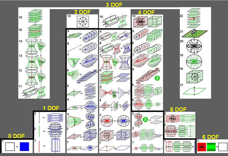
The above image contains the topologies of all flexures that contain are in series or parallel. This was the work of Jon Hopkins for his Master's and his PhD theses. Before FACT, generating flexure concepts was a matter of experience, creativity, and divine inspiration. I'll briefly explain how it works, but for a more detailed explanation, look into his papers (linked below.)
First identify the desired degrees of freedom, pick the column from the chart that has the correct number of degrees of freedom. Then find a topology that is appropriate for the specific degrees of freedom that you need. If it is under the black boundary in the chart, then it is in what's called the "parallel pyramid." That is, the topology forms a structure that exhibits all of the degrees of freedom in one flexure arrangement. This is usually preferred because it is often the simplest and most compact design. Designing parallel flexures are covered in these two papers: part 1 and part 2. Part 1 covers FACT theory and part 2 covers implementing FACT in practice. A serial flexure design is necessary when there is no parallel flexure arrangement that meets the desired degrees of freedom (e.g. 3DOF translation). Serial flexures are covered here.
Red lines indicate freedom and blue lines indicate constraint. Green lines indicate screws and orange lines (not shown) indicate wrenches. The details of screws and wrenches are beyond the scope of this entry; for more information, see Hopkins' Master's thesis.
FACT flexures are great, but the theory doesn't always work in practice. There are typically constraints on size, natural frequency, manufacturability, etc. These real-world constraints will help you pick a flexure design from the topology. Also, these constraints are going to guide the modeling and FEA that you'll do later. One real-world constraint is symmetry. Redundant flexures may need to be added to ensure that if the flexure heats up or cools down, the thermal expansion of the flexures does not affect the position of the output stage.
3.5 Transmission Theory
Transmission theory is something that I developed based on a paper by Jon Hopkins and Bob Panas for designing flexures that transform an input motion into an output motion of a different type, transmission ratio, or axis. For more information, see Chapter 2 of my Master's thesis.
4 Range of motion
The flexures have a finite length, therefore they have a finite range of motion. Further, the flexures are designed to operate below a critical stress (yield stress for ductile materials, and fracture strength for brittle materials), which thus limits the range of motion. The range of motion may be found by relating the critical stress to the bending moment of the beams, relating the bending moment to the applied load, and relating the load to displacement via stiffness. This leads to an equation for range of motion for simple cases of translation: \[\frac{\delta_\text{max}}{L} \sim \left( \frac{\sigma_\text{max}}{E} \right) \left(\frac{L}{h} \right), \]
where $\delta_\text{max}$ is the maximum displacement, $\sigma_\text{max}$ is the maximum allowable stress, $E$ is the Young's Modulus of the material $L$ is the beam length, and $h$ is the beam thickness in the bending direction. The exact equation includes a constant of proportionality that depends on the specific arrangement of beams. For most metals, $\sigma_\text{max}/E \sim 10^{-3}$, and for most plastics $\sigma_\text{max}/E \sim 10^{-2}$. Typically $L/h \sim 100$. If $L/h < \sim 10$, beam theory no longer applies, and if $L/h > 100$, then buckling becomes a more significant issue. The thickness to width ration is typically about 10 for good blade flexure constraint. Thus, for metal flexures $\delta_\text{max} \sim 0.1L$. This result can be used to generate dimensions that are in the right ballpark. Take an example of a translation flexure with a desired range of motion of $\pm$0.25 inches. For a 4-bar translation flexure, a good place to start would be with metal flexures that are about 2.5 inches long, 0.025 inches thick made out of stock that is about 0.25 inches thick. This is not optimal, but is in the right order of magnitude. Also, it's always a good idea to implement hard-stops so that the flexure is ensured to not travel too far.
5 Stiffness
The actuator provides a limited load, thus a maximum DOF stiffness is required to achieve the desired range of motion. Flexures are designed to minimize stiffness in their DOF and maximize stiffness in DOC. Translational stiffness ratios are often represented by a stiffness ellipsoid. Large networks of beams may have their stiffness represented by stiffness matrices. They may also be represented by homogenous transformation matrices (HTMs). More generally, the stiffness of a structure may be found by the Principle of Virtual Work. There are also many beam bending shortcuts that may be used, including putting springs in series or parallel. The stiffness of flexure modules have been explored in a paper by Shorya Awtar et. al. There are also closed-form nonlinear models of flexure stiffness.
The behavior of beams are well understood, but here are a couple of useful equations: stiffness, buckling, and stress. \[k = \frac{CEI}{L^3},\] where $I$ is the second moment of area given by \[I = \iint\limits_A y^2 \mathrm{d}A\]
And of course, \[ \sigma = \frac{Mc}{I}. \]
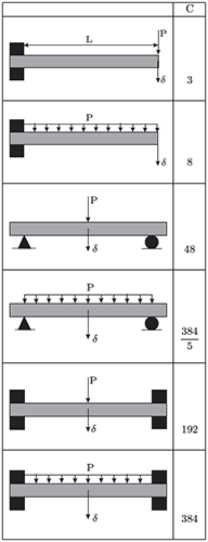
The critical buckling load is given by \[P_{cr} = \frac{\pi^2 EI}{L_e^2}\] Use the chart below to find the effective length, $L_e = KL$. This chart was adapted from the Steel Construction Manual from the American Institute of Steel Construction.

 The fact that stiffness changes as a function of displacement is important for flexure design because the stiffness in the DOC may change dramatically. This is covered in Design Principles for Precision Mechanisms and in Shorya Awtar's PhD thesis.
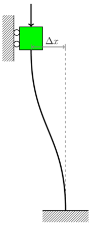
The stiffness of an axially loaded straight beam is
\[ k_{a0} = \frac{EA}{L},\]
where $A$ is the cross-sectional area. The axial stiffness changes when the beam deflects by an amount $\Delta x$, becoming
\[k_a (\Delta x) = k_{a0} \frac{1}{1+ \frac{3}{175}\left( \frac{\Delta x}{h} \right)^2}. \]
The axial stiffness drops off dramatically after about 1 beam thickness, and after about 7 beam thicknesses, the axial stiffness is approximately equal to the transverse stiffness. Thus, when designing flexures, the constraint stiffness should be measured over the full range of displacements in the degree(s) of freedom.
The fact that stiffness changes as a function of displacement is important for flexure design because the stiffness in the DOC may change dramatically. This is covered in Design Principles for Precision Mechanisms and in Shorya Awtar's PhD thesis.
The stiffness of an axially loaded straight beam is
\[ k_{a0} = \frac{EA}{L},\]
where $A$ is the cross-sectional area. The axial stiffness changes when the beam deflects by an amount $\Delta x$, becoming
\[k_a (\Delta x) = k_{a0} \frac{1}{1+ \frac{3}{175}\left( \frac{\Delta x}{h} \right)^2}. \]
The axial stiffness drops off dramatically after about 1 beam thickness, and after about 7 beam thicknesses, the axial stiffness is approximately equal to the transverse stiffness. Thus, when designing flexures, the constraint stiffness should be measured over the full range of displacements in the degree(s) of freedom.
6 Load Capacity
The load capacity of the flexures is limited by strength and stability. The stress should be below an critical level when the maximum load is applied. Also, the beams may buckle under the maximum load. Both strength and stability should be modeled and characterized by FEA. Hard-stops should be implemented to ensure that the load capacity is not exceeded.
7 Dynamics
The flexure also needs to be designed to achieve the appropriate mode shapes and frequencies. The mode shapes give an idea of the degrees of freedom of the system, but they are also affected by the mass distribution. The flexure may be excited by many sources, including actuator noise, electrical noise, sudden impulses, etc. It is important that these frequencies are not exciting an undesirable resonant mode. Also, flexures are lightly damped ($\zeta \approx 0.01$) which means that the vibrations take a long time to die out, and that they have a large dynamic amplification factor at resonance. The dynamic amplification factor is a ratio of the dynamic displacement ($z_\text{dynamic}$) to the static displacement ($z_\text{static}$), which changes with frequency ($\omega$). This animation may be viewed for a more intuitive understanding of how the displacement changes with frequency. For a 1-DOF underdamped second-order system, 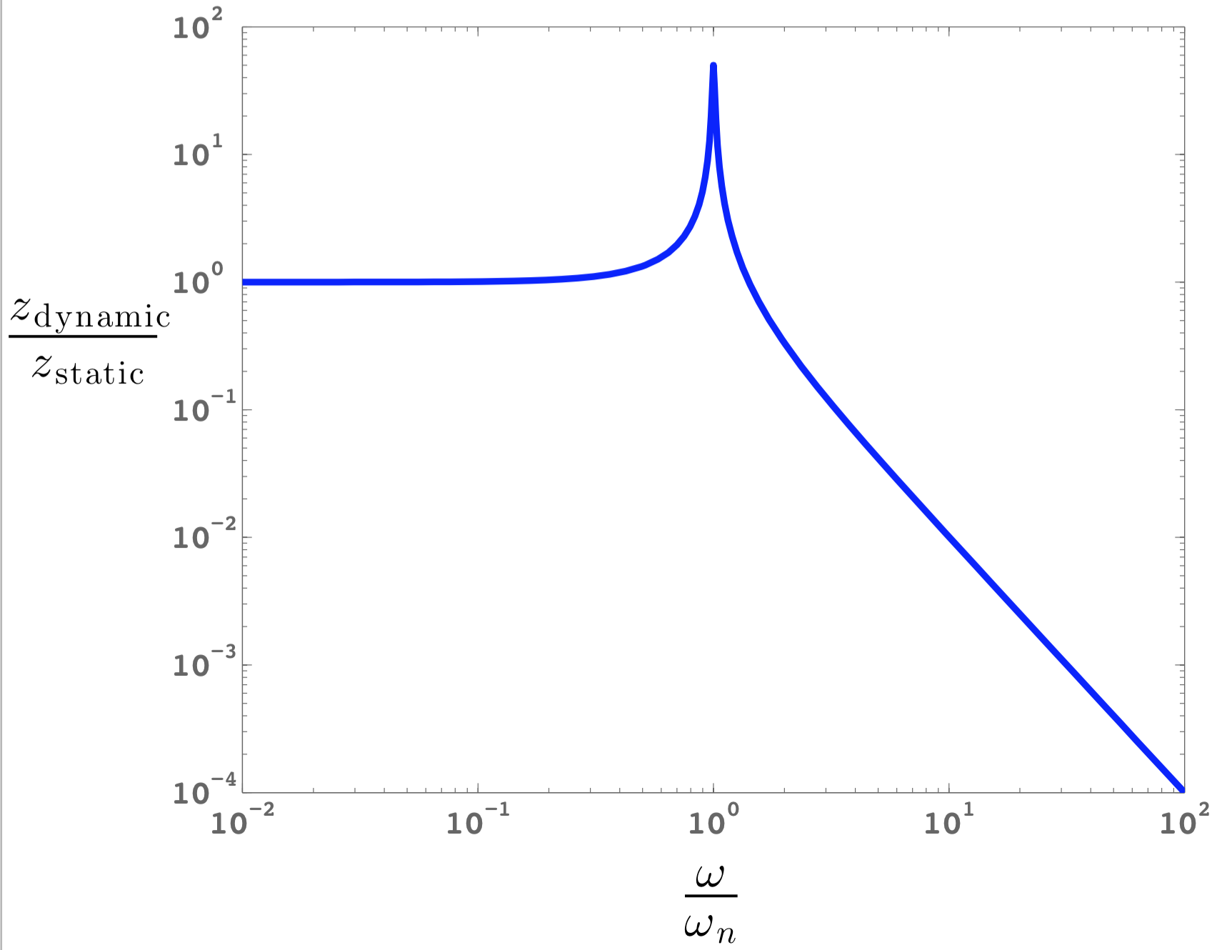 \[ \frac{z_\text{dynamic}}{z_\text{static}} = \frac{1}
{ \sqrt{\left[1- \left( \frac{\omega}{\omega_n} \right)^2 \right]^2 + \left[ 2\zeta \frac{\omega}{\omega_n} \right]^2 }}, \]
where $\zeta$ is the damping ratio and $\omega_n$ is the natural frequency given by
\[\zeta = \frac{c}{2\sqrt{km}},\hspace{10pt} \omega_n = \sqrt{\frac{k}{m}}, \]
where $m$ is the mass, $c$ is the dashpot constant, and $k$ is the spring stiffness. The maximum dynamic amplification factor occurs at $\omega_\text{peak}$:
\[\omega_\text{peak} = \omega_n \sqrt{1-2\zeta^2} \approx \omega_n,\]
and
\[\left(\frac{z_\text{dynamic}}{z_\text{static}} \right)_\text{max} = \frac{1}{2\zeta \sqrt{1-\zeta^2}} \approx \frac{1}{2\zeta}.\]
Meso-scale (10s cm-scale) flexures typically have $\zeta \approx 0.01$, so when they are actuated at resonance, they have a dynamic amplification factor $\approx 50$. There are some ways to fix this: actuate it at a much higher frequency (or move the resonant frequency much lower) to make the dynamic amplification factor < 1, and the damping may be increased by using a thin film of bearing grease between the output stage and ground. See Chapter 4 of my Master's thesis for a way to measure the damping ratio by taking the log decrement.
\[ \frac{z_\text{dynamic}}{z_\text{static}} = \frac{1}
{ \sqrt{\left[1- \left( \frac{\omega}{\omega_n} \right)^2 \right]^2 + \left[ 2\zeta \frac{\omega}{\omega_n} \right]^2 }}, \]
where $\zeta$ is the damping ratio and $\omega_n$ is the natural frequency given by
\[\zeta = \frac{c}{2\sqrt{km}},\hspace{10pt} \omega_n = \sqrt{\frac{k}{m}}, \]
where $m$ is the mass, $c$ is the dashpot constant, and $k$ is the spring stiffness. The maximum dynamic amplification factor occurs at $\omega_\text{peak}$:
\[\omega_\text{peak} = \omega_n \sqrt{1-2\zeta^2} \approx \omega_n,\]
and
\[\left(\frac{z_\text{dynamic}}{z_\text{static}} \right)_\text{max} = \frac{1}{2\zeta \sqrt{1-\zeta^2}} \approx \frac{1}{2\zeta}.\]
Meso-scale (10s cm-scale) flexures typically have $\zeta \approx 0.01$, so when they are actuated at resonance, they have a dynamic amplification factor $\approx 50$. There are some ways to fix this: actuate it at a much higher frequency (or move the resonant frequency much lower) to make the dynamic amplification factor < 1, and the damping may be increased by using a thin film of bearing grease between the output stage and ground. See Chapter 4 of my Master's thesis for a way to measure the damping ratio by taking the log decrement.
Looking at the system response in the frequency domain is important for responding to noise of a known frequency (or range of frequencies) e.g. 60 Hz noise from plugging a device into a wall. It is often more useful to look at the time response for sudden excitations, like impulses or steps. The step response and impulse response can show how long it takes for noise to die out, and the amount of overshoot.
Also, plastics are viscoelastic, so other dynamic issues to consider are creep and stress relaxation. This behavior can be quite problematic for a micro-positioning stage with a force-controlled actuator, for example. The flexures themselves may not be made from plastic, but viscoelasticity from epoxy can affect the overall dynamics.
For MEMS resonators and oscillators, the dynamics can be quite complex. They involve many more damping mechanisms, including thermoelastic damping (the ultimate limit of damping in a material), phonon-phonon scattering, anchor loss, surface effects, and electrical losses. They may also be thermo-mechanically actuated, so the thermal time-constant is important as well. See papers by Marc Weinberg, Amy Duwel, and Rob Candler on MEMS damping mechanisms, and see papers by Shi-Chi Chen and Martin Culpepper on thermo-mechanical actuation.
8 Fatigue
Fatigue is important to ensure that the flexure has a long ("infinite") life. The maximum stress should be lower than the endurance limit if the flexure is made of steel (preferably stainless so it doesn't rust.) The flexures shown in lab experiments are often made from aluminum even though aluminum has no endurance limit (i.e. it will break eventually.) This is because aluminum is easy to machine and in a lab setting, the flexures are often loaded for <1000 cycles, which means that fatigue failure is not often an issue. Implementing flexures in commercial devices however requires fatigue analysis. A rule of thumb is that if $\sigma < \sigma_y /3$, then the flexure will last $>10^6$ cycles. See Shigley's Mechanical Engineering Design for more information about fatigue analysis.
9 Repeatability
Flexures alone may have Å-level repeatability because they are limited by the motions of atomic dislocations. Thus, to maximize precision, $\sigma \ll \sigma_y$. A good rule of thumb is to keep $\sigma < \sigma_y/3$. The repeatability of the motion of the output stage is limited by the whole system, including the actuator (precision in magnitude and direction), the sensor precision, material hysteresis (preferably single crystal) and the constraints (bolted joints). If the flexures are assembled with bolted joints, there may be hysteresis caused by micro-slip at the interface. Micro-slip is a friction-based phenomenon where parts move by ~10s of microns at a force < $\mu_\text{static} N$. The surface asperities need to be crushed to mitigate micro-slip, so the compressive stress should be high. This may be achieved by tightening the bolts (high force), and placing the bolted joints on washers (small area). This micro-slip may be measured by applying a required load to the flexure and measuring the displacement of the bolted joint ("ground").
10 Error Budget
The flexures are not perfect and the errors from various sources should be bounded. The flexures are sensitive to geometric errors (length, thickness, angles, etc.) These geometric errors may be initial imperfections caused by fabrication errors. Geometric errors may also result from thermal expansion. The flexures are thin relative to the rest of the structure, so they have a relatively small thermal time constant. There may also be inaccuracy in the magnitude and direction of the actuator. The sensor accuracy must also be taken into account. The material used may not have the average material properties. For example, materials that have been rolled (e.g. sheet metal) are anisotropic (i.e. the stiffness will depend on direction). These errors should be taken into account when modeling the flexures.
11 Optimization
The flexure may be optimized with several goals in mind: minimizing DOF stiffness, maximizing DOC stiffness, maximizing load capacity, distributing the mass and altering the damping to achieve optimal dynamics, minimizing stress, maximizing range of motion, etc. There are several ways to perform numerical optimization, especially with a tools like MATLAB or Mathematica. Also, SolidWorks has Design Studies for optimization. Ultimately, remember that the design is fine as long as it meets the functional requirements.
12 Fabrication
Flexures may be fabricated by wire EDM, Waterjet, CNC Mill, or laser cutting. Wire EDM is preferred because of its precision (~$\pm$1 micron). Waterjetting has a tolerance of $\pm$0.005 inches ($\pm$127 microns). CNC milling flexures is tricky because the cutting forces deflect the thin beams, so the tolerances I've achieved are similar to the Waterjet. One trick that I have yet to try is to fill the open areas of the flexure with wax to stiffen the overall structure. Laser cutting flexures can be especially troublesome because, for thin enough beams, the heat affected zone can cause the beams to thermally expand and stick to the opposing sidewall. The flexures may be broken when removing them from the laser cutter. For MEMS, the fabrication process is complex and error-prone. See Microsystem Design by Senturia for more information. Flexure stages may also be bought from the following vendors: Motus Mechanical, Riverhawk, Thorlabs, and Bal-Tec.