Introduction
The purpose of this website is to
explain how to extract information on the heterogeneity of a system from
multiple particle tracking data. We begin with a brief overview of multiple
particle tracking (MPT) and microrheology before moving on to the topic
of heterogeneity. More extensive introductions to MPT can be found in
the paper by Crocker & Grier (1996) and the website "Particle
tracking using IDL", both referenced here .
.
What is multiple
particle tracking?

Multiple Particle Tracking is a technique
that allows you to simultaneously track several micron-sized particles
using video microscopy. You record video microscopy movies of micro-spheres
undergoing Brownian motion, and using the image processing software given
on the website "Particle tracking using IDL" linked here,
you can extract from the movies the individual trajectories of the particles.
This is illustrated in the movie on the right (click on the picture to
launch the movie) where you can see the thermal motions of 1.1 μm-diameter
fluorescent spheres mixed in water (left-hand side of the movie), and
the trajectories I extracted from the same movie (right-hand side). Note
that trajectories are measured individually (and I used different colors
to display them). Also note that some particles are moving out of focus,
which ends their tracking, and come back in focus, which starts a new
trajectory (even if it is potentially the same particle).
How do the
data look like?
The output of multiple particle tracking
are trajectories. Commonly, these trajectories are 2D, and are stored
in an array that looks like that:
The 4th column is the trajectory identification number i = 0, 1, 2, ...; the 3rd is the time index j = 0, 1, 2, ...; the first two columns give the corresponding positions in the (x,y) imaging plane,
of the trajectory labelled i at the time j. Eventually more information is extracted from the movie processing but it is not important for what we want to do here.
| x | y | time j | id i |
| 42.6914 | 81.6781 | 0.00000 | 0.00000 |
| 43.5721 | 82.8166 | 1.00000 | 0.00000 |
| 42.4250 | 81.9106 | 2.00000 | 0.00000 |
| 44.0587 | 83.6478 | 3.00000 | 0.00000 |
| 41.8534 | 83.0542 | 4.00000 | 0.00000 |
| 301.995 | 158.851 | 2.00000 | 1.00000 |
| 301.542 | 156.749 | 3.00000 | 1.00000 |
| 300.578 | 157.351 | 4.00000 | 1.00000 |
| 302.855 | 157.835 | 5.00000 | 1.00000 |
| 299.127 | 159.383 | 6.00000 | 1.00000 |
| . | . | . | . |
| . | . | . | . |
| . | . | . | . |
The 4th column is the trajectory identification number i = 0, 1, 2, ...; the 3rd is the time index j = 0, 1, 2, ...; the first two columns give the corresponding positions in the (x,y) imaging plane,
| rij = ( xij , yij ) |
of the trajectory labelled i at the time j. Eventually more information is extracted from the movie processing but it is not important for what we want to do here.
An important
quantity: the mean-squared displacement (msd)
The mobility of a colloidal tracer
reflects the mechanical properties of the microenvironment it is embedded
in. Analyzing data for a single particle, or groups of particles, allow
us to quantify the mechanical properties of micro-scale environments.
Since they are stochastic processes, the relevant physical observables
we are interested in are averages. For reasons I will discuss
in the next paragraph, an averaged quantity that is
often calculated is called the mean-squared displacement. I will explain
how to calculate this quantity in the next section,
but I give here its generic formula:
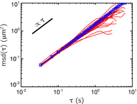
where r(t) is is the position of the particle at time t, and τ is the lag time between the two positions taken by the particle used to calculate the displacement Δr(τ) = r(t+τ) - r(t). The average <...> designates a time-average over t and/or an ensemble-average over several trajectories. But at this point, it is important to understand that the mean-squared displacement can be calculated from a single trajectory by only performing a time average. If I calculate the msd vs. τ for the Brownian particles in water I had tracked in the movie linked above, I find the results shown in the figure on the left. Again, I will give more details later on how I calculated this msd. Here I performed a time and ensemble average over all measured trajectories to obtain the blue points. Each red curve is a time-average calculation over a single trajectory. These red curves are affected by a greater statistical uncertainty than the blue curve, but all curves follow the same trends. The log-log plot shows in particular that in that case, the msd varies linearly with the lag time, msd(τ) ∝ τ. This is a characteristic of the Brownian motion observed in a purely viscous (or Newtonian) fluid, such as water. We can push further this qualitative observation by using the formalism of microrheology.
| msd(τ) = <Δr(τ)2> = <[r(t+τ) - r(t)]2> |
where r(t) is is the position of the particle at time t, and τ is the lag time between the two positions taken by the particle used to calculate the displacement Δr(τ) = r(t+τ) - r(t). The average <...> designates a time-average over t and/or an ensemble-average over several trajectories. But at this point, it is important to understand that the mean-squared displacement can be calculated from a single trajectory by only performing a time average. If I calculate the msd vs. τ for the Brownian particles in water I had tracked in the movie linked above, I find the results shown in the figure on the left. Again, I will give more details later on how I calculated this msd. Here I performed a time and ensemble average over all measured trajectories to obtain the blue points. Each red curve is a time-average calculation over a single trajectory. These red curves are affected by a greater statistical uncertainty than the blue curve, but all curves follow the same trends. The log-log plot shows in particular that in that case, the msd varies linearly with the lag time, msd(τ) ∝ τ. This is a characteristic of the Brownian motion observed in a purely viscous (or Newtonian) fluid, such as water. We can push further this qualitative observation by using the formalism of microrheology.
Microrheology
The mean-squared displacement characterizes
the dynamics of the particles we are tracking: it shows the amplitude
of the particle's motion at a characteristic time given by τ.
These dynamics are related to the mechanical properties of the medium
in which the particles are moving. For example, particles in a continuum
viscous material will have a mean-squared displacement growing linearly
with the lag time, but the more viscous it is, the slower will be the
rate of growth of msd(τ)
vs. τ. In particular,
in a viscous fluid we have:
where d is the dimensionality of the track (d=2 here in 2-dimensions) and D = kT / (6πηa) is the diffusion coefficient. In this formula, k is the Boltzmann constant, T is the temperature, η is the viscosity of the fluid and a is the radius of the particles. From the blue curve of the plot shown above, we calculate
which is the accepted value for the viscosity of water at 23°C, as compared to tabulated values obtained using different techniques. This type of calculations lies in the framework of (passive) microrheology, where the motion of Brownian particles can be used to measure the mechanical properties of the material they are embedded in. Generalizations of this relation exist and can be used to calculate the complex shear modulus spectrum from msd(τ) to characterize viscoelastic behavior of the material in which particle tracking was performed. For the purpose of this tutorial, it is important to understand that individually calculated msd's (such as the red curves in this plot) can also be used to perform local microrheological measurements.
| msd(τ) = 2dDτ |
where d is the dimensionality of the track (d=2 here in 2-dimensions) and D = kT / (6πηa) is the diffusion coefficient. In this formula, k is the Boltzmann constant, T is the temperature, η is the viscosity of the fluid and a is the radius of the particles. From the blue curve of the plot shown above, we calculate
| D = 0.43 μm2.s-1 ⇒ η = 9.2×10⁻⁴ Pa.s |
which is the accepted value for the viscosity of water at 23°C, as compared to tabulated values obtained using different techniques. This type of calculations lies in the framework of (passive) microrheology, where the motion of Brownian particles can be used to measure the mechanical properties of the material they are embedded in. Generalizations of this relation exist and can be used to calculate the complex shear modulus spectrum from msd(τ) to characterize viscoelastic behavior of the material in which particle tracking was performed. For the purpose of this tutorial, it is important to understand that individually calculated msd's (such as the red curves in this plot) can also be used to perform local microrheological measurements.