Scenes and objects database

One of the major problems when developing object detection algorithms is the lack of labeled data for training and testing many object classes. The goal of this database is to provide a large set of images of natural scenes (principally office and street scenes), together with manual segmentations/labelings of many types of objects, so that it becomes easier to work on general multi-object detection algorithms.

This database was created by Antonio Torralba, Kevin P. Murphy and William T. Freeman.

Downloads

For getting the database and Matlab code follow the next link: Download Database

If you find this dataset usefull, help us to build a larger dataset of annotated images (which will be made available very soon) by using the web annotation tool written by Bryan C. Russell at MIT:

Go to the labeling tool

Overview of the database content

Here there are some of the characteristics of the database:

This database includes indoor and outdoor objects in office and urban environments. The database contains thousands of images (static and sequences), with about 2500 annotated frames.
The database provides annotations for more than 30 objects in context.
The database is organized in folders. Each folder contains images from different places. The interest of this organization is that you can use a set of folders for training and another subset for testing, to be sure that both training and test sets are independent.
Objects are labeled with polygons. The polygons provide a good approximation to the outline of the object (this is more than a simple bounding box).
Some objects provide additional information like point of view.
Images are also label according to scene information. Some of the frames provide specific place information (ex. Office 225, corridor 2 building 200, etc.) and for most of the images in the dataset there are generic scene names (office, street, corridor, etc.)
Images come from different sources (webcam, digital cameras, and images from the web).
The database contains static pictures and sequences.
We provide a set of Matlab tools to read the annotation files and do queries to the dataset.

Limitations:

The annotations are sparse. Not all the instances of an object class are labeled across all the images.
Some frames have dense labeling (almost all the pixels are labeled) and some other frames have only one or two objects labeled.
Although most of the polygons try to follow the object outline, some annotations are lousy.

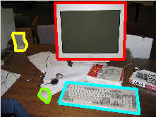
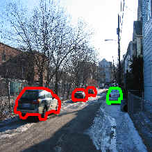
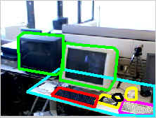
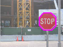
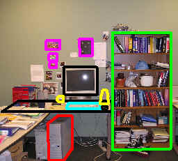
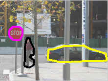
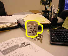
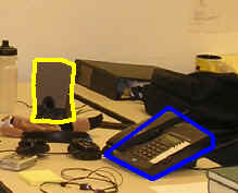
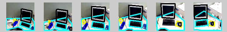
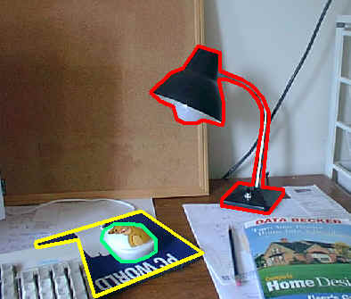
The following images show some example of annotated frames (static frames and sequences):

Each labeled image in the database is associated with an annotation ASCII file. This is an example of one annotation file:

# - List of Polygons

size {427 640 3}

makePolygon {Polygon 1} mouse {457 279 464 281 471 281 470 277 464 276 460 276}

makePolygon {Polygon 2} deskFrontal {534 276 19 336 19 308 264 283 475 261}

makePolygon {Polygon 3} poster {545 122 578 124 575 188 544 188}

makePolygon {Polygon 4} keyboard {384 281 400 291 453 283 439 276}

makePolygon {Polygon 5} cpu {254 230 233 224 203 225 204 289 228 298 257 296}

makePolygon {Polygon 6} screenFrontal {130 237 132 295 199 290 197 235}

view {270 -999}

makePolygon {Polygon 7} light {442 19 468 11 591 30 562 37}

Objects

The next table is a list of all the object labels used in the annotations. Some of the labels correspond to parts of objects. The objects denoted with a (*) are interesting object for training detectors (interesting means that there are a reasonable number of annotated instances and some control for the variability of the object appearance):

'apple' (*)
'bicycle'
'bicycleSide'
'bookshelf'
'bookshelfFrontal' (*)
'bookshelfPart'
'bookshelfSide'
'bookshelfWhole'
'bottle' (*)
'building'
'buildingPart'
'buildingWhole'
'can' (*)
'car' (*)
'carFrontal' (*)
'carPart'
'carSide' (*)
'cd' (*)
'chair'
'chairPart'
'chairWhole' (*)
'coffeemachine'
'coffeemachinePart'

'coffeemachineWhole' (*)
'cog'
'cpu' (*)
'desk'
'deskFrontal' (*)
'deskPark'
'deskPart'
'deskWhole'
'donotenterSign' (*)
'door'
'doorFrontal' (*)
'doorSide'
'filecabinet'
'firehydrant' (*)
'freezer'
'frontalFace' (*)
'frontalWindow'
'head' (*)
'keyboard' (*)
'keyboardPart'
'keyboardRotated'
'light' (*)
'mouse' (*)

'mousepad' (*)
'mug' (*)
'onewaySign' (*)
'paperCup' (*)
'parkingMeter' (*)
'person'
'personSitting'
'personStanding'
'personWalking' (*)
'poster' (*)
'posterClutter'
'pot' (*)
'printer'
'projector'
'screen'
'screenFrontal' (*)
'screenPart'
'screenWhole' (*)
'shelves'
'sink'
'sky'
'sofa'

'sofaPart'
'sofaWhole'
'speaker' (*)
'steps'
'stopSign' (*)
'street'
'streetSign'
'streetlight'
'tableLamp' (*)
'telephone' (*)
'torso'
'trafficlight' (*)
'trafficlightSide'
'trash'
'trashWhole' (*)
'tree'
'treePart'
'treeWhole'
'wallClock'
'watercooler'
'window'

Regions:

'buildingRegion'
'roadRegion'
'skyRegion'
'treeRegion'
'walksideRegion'

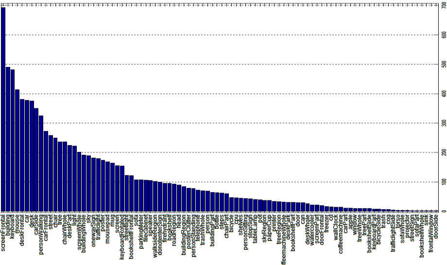
Here there is a histogram of counts for each labeled object (or parts of objects). The vertical axis is the number of labeled instances (resolution varies).

Places and scenes

The frames are also labeled according to scene type (office, corridor, street, conference room, etc.)

Structure of the annotation files

This is an example of one annotation file:

# - List of Polygons

size {427 640 3}

makePolygon {Polygon 1} mouse {457 279 464 281 471 281 470 277 464 276 460 276}

makePolygon {Polygon 2} deskFrontal {534 276 19 336 19 308 264 283 475 261}

makePolygon {Polygon 3} poster {545 122 578 124 575 188 544 188}

makePolygon {Polygon 4} keyboard {384 281 400 291 453 283 439 276}

makePolygon {Polygon 5} cpu {254 230 233 224 203 225 204 289 228 298 257 296}

makePolygon {Polygon 6} screenFrontal {130 237 132 295 199 290 197 235}

view {270 -999}

makePolygon {Polygon 7} light {442 19 468 11 591 30 562 37}

The size of the image:

size {427 640 3}

One object is described by a polygon:

makePolygon {Polygon 1} mouse {457 279 464 281 471 281 470 277 464 276 460 276}

The field "labels" allows to add additional information to describe an object. For instance, in the case of a "face", we might want to add information like the gender or the identity. The labels can be arbitrary:

makePolygon {1} frontalFace {139 136 206 136 146 219 197 220 110 126 150 126 188 127 225 124 107 141 123 140 152 140 191 139 222 138 234 140 172 173 161 180 183 180 171 204 171 240 171 271}

labels {{gender:male}{identity:pepe}{label 3:property 3}{label 4: property 4}}

We can then query to find objects with specific labels:

keys = queryDB(DB, 'findObject', 'frontalFace', 'findLabel', 'gender=male');

MATLAB tools for handling the annotation files

We have developed some MATLAB tools for using the database. The first set of function allows to read and create annotation files. The second set of function provides higher-level functions for indexing the annotations.

Reading and plotting images

There are four basic functions for reading, writing and plotting the annotation files:

pfRead: Opens a file and returns a struct array containing the fields read from the file.
pfWrite: Creates an annotation text file.
pfGet: Extracts the polygons that are drawn in a figure.
pfDraw: Draw in the current axis all the polygons contained in pf.

All these four functions describe the polygons on an image using a struct array:

pf(:).class
pf(:).polygon
pf(:).vertices
pf(:).view
pf(:).labels

Queries to the database

There are some basic MATLAB tools to make queries to the database in order to locate the frames that contain specific objects or scenes.

1) First you have to create the database.

DB = makeDB('C:/images', 'C:/anno', 'C:/places')

The arguments are the directories in which the images, object annotations and place labels are stored.

The result of this function is the struct 'DB' which is an index for the database. This operation will take some time but you only have to do it once. Once is done, you can store the struct DB somewhere for future use.

2) Searching the database

>> load DB

>> keys = queryDB(DB, 'findObject', 'screenFrontal');

keys =

1x560 struct array with fields:
frame
objects

'keys' are pointers to frames and objects within each frame. For instance:

>> keys(1)

ans =

frame: 318
objects: 3

This indicates that the first image that contains a 'screenFrontal' is frame number 318, and the object is number 3 in the annotations. Therefore:

>> DB.frame(318).objects(3)

ans =

className: 'screenFrontal'
vertices: [2x4 double]
center: [527.4829 261.4052]
area: 139415
bbox: [4x1 double]
view: [2x1 double]

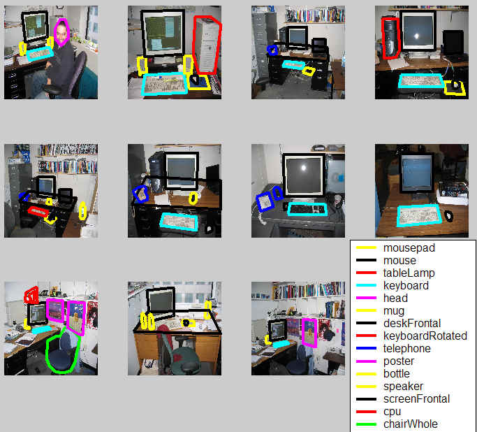
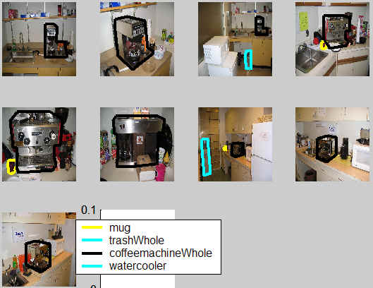
You can visualize some of the images with:

>> showImages(DB, [keys(1:10).frame])

Some other query examples:

>> keys = queryDB(DB, 'findObject', 'coffeemachineWhole', 'findObject', '~freezer', 'findObject', '~desk*');

>> showImages(DB, keys.frame);

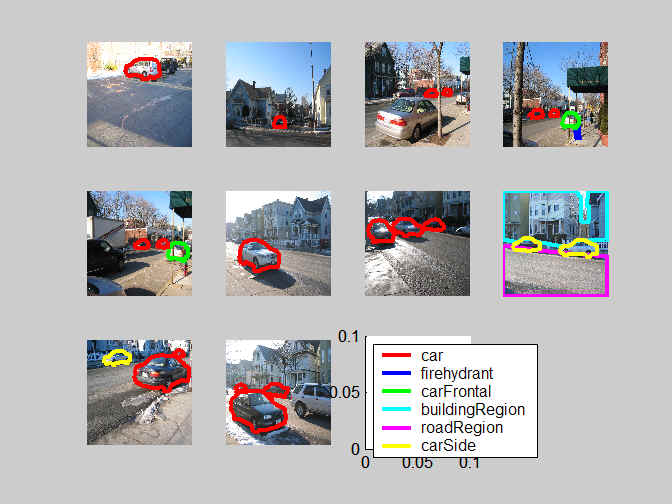
>> keys = queryDB(DB, 'findObject', 'car*');
>> showImages(DB, [keys(1:10).frame])

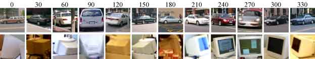
3) Searching points of views

For some objects, we have also labeled the point of view. The labeling of the point of view is done by adding one line into the annotation file, just after the object polygon. For instance:

makePolygon {Polygon 6} screenFrontal {130 237 132 295 199 290 197 235}

view {270 -999}

Here there are some examples of objects and the views used:

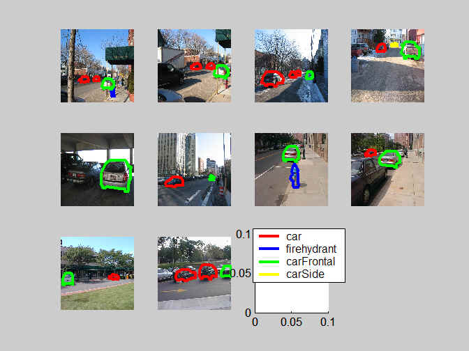
It is possible to find objects in the database using the point of view as a query argument:

>> keys = queryDB(DB, 'findObject', 'car*', 'findAzimuth', 90);

>> showImages(DB, [keys(1:10).frame])

This returns frames that contain views of backs of cars (and other objects too):

4) Querying folders

Using folder names in the query is useful to create training and test datasets that are independent. Here we give some examples of useful queries:

Get all sequences:

keys = queryDB(DB, 'findFolder', 'seq');

Get all static pictures:

keys = queryDB(DB, 'findFolder', 'static');

Get all images retrieved from the web:

keys = queryDB(DB, 'findFolder', 'web');

Get all images from building 200 (old AI-Lab building):

keys = queryDB(DB, 'findFolder', 'bldg200');

Get all images from Stata center (new CSAIL building):

keys = queryDB(DB, 'findFolder', 'stata');

Queries can be combined to locate instances of an object within a set of images:

keys1 = queryDB(DB, 'findObject', 'frontalScreen', 'findFolder', 'bldg200');

keys2 = queryDB(DB, 'findObject', 'frontalScreen', 'findFolder', 'stata');

Now, keys1 and keys2 are pointers to images containing "screens" taken in different buildings and therefore, provide a possible split in training and test sets.

5) Searching scenes

keys = queryDB(DB, 'findLocation', '400_fl_608');