

5.4.4 System Performance Measures (Infinite Line Capacity)Now that we know how to obtain the steady-state probabilities of the hypercube model, it is natural to inquire how to use these probabilities to obtain values of useful system performance measures. Workloads. We can immediately obtain the workloads of
the individual servers. The workload
These results check (to four significant figures) with the
requirement that the average workload Interatom dispatch frequencies. For virtually all non-workload-oriented performance measures it is necessary to compute fnj Let Enj For instance, in our three-server example, E21 =
{001, 101} and E11 = {000, 010, 100, 110}. If the
system is in any state in the set Enj, then the
fraction of service requests that result in the dispatch of unit
n to atom j is
The term fnj[2] is equal to the product of three terms: (1) the probability that a randomly arriving service request incurs a queue delay; (2) the conditional probability that the request originated from atom j, given it incurs a queue delay; and (3) the conditional probability that the request results in the dispatch of unit n, given that it originates from atom j and incurs a queue delay. Clearly, a queue delay will be incurred by any request arriving while all N response units are busy, and thus the first term is
The second term is equal to the fraction of calls (
and thus
Given that we now know how to calculate the fnj's from the state probabilities, we can immediately obtain several related performance measures of interest:
We illustrate each of these computations with our three-server
example. First computing the additive term associated with queued
requests, we note
that P'Q = 0.23684 and thus
fnj[2] =
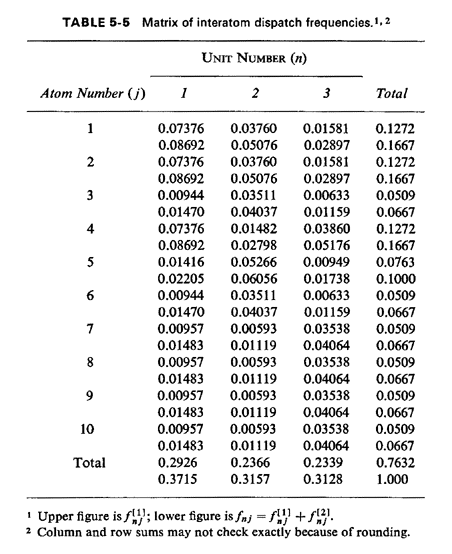
In other words, about 8.7 percent of all service requests are the type that result in unit 1 being sent to atom 1. The full set of fnj's is displayed in Table 5-5. Employing (5.36), the fraction of responses that are interresponse area is 0.43529. This figure checks with our intuition which might argue, roughly, that the fraction of intraresponse area responses would be equal to the average availability (50 percent) plus one-third the probability of incurring a queue delay (P'Q = 0.23684), yielding a fraction of intraresponse area responses equal to 0.57895, or a fraction of interresponse area responses equal to 0.42105. The actual figure of 0.435 is larger than that conjectured due to workload imbalances, as we will argue in Section 5.6. 
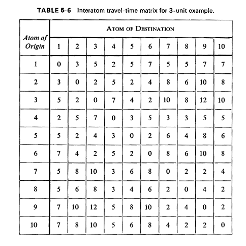
Employing (5.37), the fraction of dispatches of unit 1 that are interresponse area is 0. 11077/0.3715 = 0.2982. Employing (5.38), the fraction of responses into response area 1 that are interresponse area responses is 0.23919/0.500 = 0.4784. Thus, we see that the unit-specific frequency of interresponse area responses can be significantly different from the response-area-specific frequency. In this case, fully (1.0 - 0.4784) x 100 percent = 52.16 percent of response area 1's workload is handled by unit 1, and thus 47.84 percent is handled by units 2 and 3. But (1.0 - 0.2982) x 100 percent = 70.18 percent of unit 1's workload is within response area 1. Travel times. Travel time is a central performance measure computed by the hypercube model. All travel times are computed from a travel-time matrix whose generic element is ,
the mean travel time from atom i to atom j. The numerical
values of the ,
the mean travel time from atom i to atom j. The numerical
values of the  ij's may reflect
complications to travel such as ij's may reflect
complications to travel such as
one-way streets, barriers, traffic conditions, and so on. Thus, the
time required to travel from i to j may not be the same as
the time to travel from j to i and thus we allow 
To compute system mean travel times, we also require knowledge of the
location of a unit when dispatched to a request. In the hypercube
framework, the geographical depiction of the "location" of a response
unit is general enough to model the fixed locations of ambulances and
emergency repair vehicles and the mobile locations of police patrol
units. This is accomplished by specifying a location matrix L =
(lnj), where lnj is the
probability that response unit n is located in atom j while available
for dispatch (or, equivalently, the fraction of available or idle
time that response unit n spends in atom j). We require
that L be a stochastic matrix (i.e., for all n, To obtain travel-time performance measures, it is necessary to compute tnj Since unit n will be located in atom k with probability lnk, we can write
To include the case of assignments from queues, we define the mean "queued request travel time,"
To interpret this expression, consider any particular service request
which incurs a queue delay. The request is generated from atom j
with probability The expression for the region-wide unconditional mean travel time can now be written
If we define  j = average travel
time to atom j j = average travel
time to atom jfollowing reasoning analogous to that above, we write
If we are interested in the mean travel time to requests in a particular primary response area, we define
Assuming response area n includes at least one atom j
with
Unfortunately, there is no known (exact) expression for the average
travel time of unit n (assuming infinite queue capacity). The
problem in deriving such an expression arises from the fact that the
unit's position when dispatched for the first time back-to-back (with no
idle time) during a system busy period is not selected from the
probability distribution of request locations
We must recognize that the term reflecting travel time to queued
requests is an overestimate which becomes asymptotically exact as the
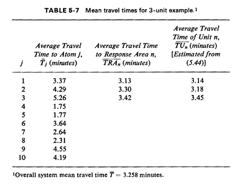
system utilization factor Returning to our 3-unit example, substitution into (5.40) yields a
mean queued request travel time 
From this information, we can compute that the overall system mean
travel time, from (5.41), is
9If the computed mean travel times in Table 5-7 are found to be inconsistent with the assumption that the mean total service time of each unit is the same known constant, then one must enter these travel times into a new computation for (unit-specific) mean service times and execute the model again to accomplish mean service time calibration (see Sec. 5.3.1). Several such executions may be necessary to achieve convergence. 
|