5.5.3 Return to the Three-Server Example
We apply the workload approximation procedure to the three-server,
10-atom example of the previous section. Recall that  = 1.5, = 1.5,  = 1, implying that = 1, implying that
 = =  /(3 x 1) = 0.5. To
initiate the procedure we need to specify the dispatch preference sets
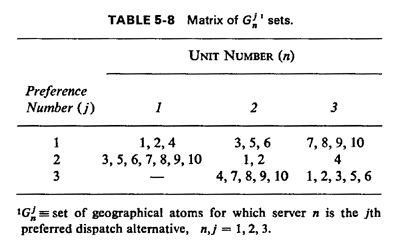
Gnj, and these are shown in Table 5-8. From
(5.48) we compute the numerical values for the three required correction
factors: /(3 x 1) = 0.5. To
initiate the procedure we need to specify the dispatch preference sets
Gnj, and these are shown in Table 5-8. From
(5.48) we compute the numerical values for the three required correction
factors:

 Q(3, ½, 0) = 1
Q(3, ½, 1) = 0.73684
Q(3, ½, 2) = 0.63158
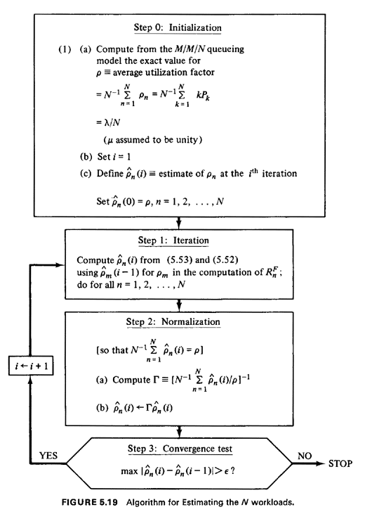
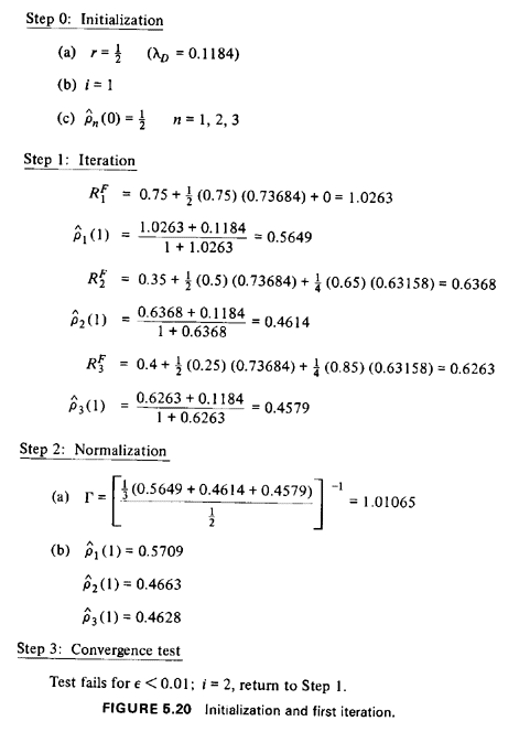
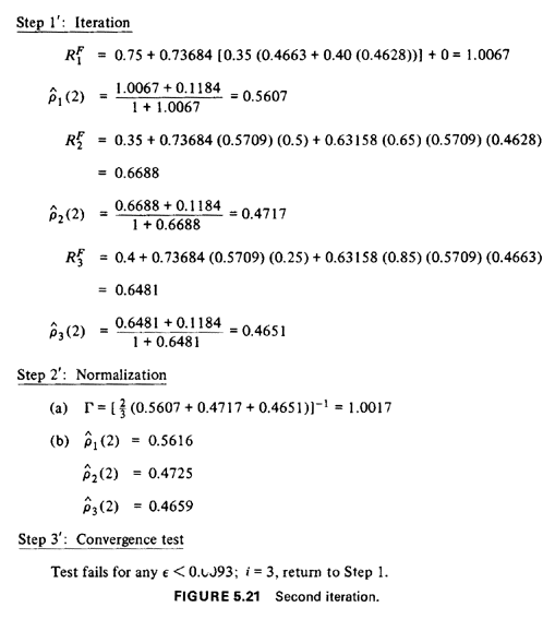
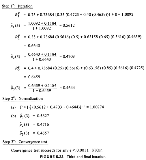
We are now ready to proceed through the steps of the algorithm. One
complete iteration of the algorithm is shown in each of Figures
5.20-5.22. As can be seen, the procedure has converged for a very
stringent convergence criterion ( = 0.0011
or greater) on the third iteration. The resulting workloads are
estimated to be = 0.0011
or greater) on the third iteration. The resulting workloads are
estimated to be  1 = 0.5627, 1 = 0.5627,  2 = 0.4716, and 2 = 0.4716, and  3 = 0.4657. The exact workloads, as
computed from the exact hypercube model, are 3 = 0.4657. The exact workloads, as
computed from the exact hypercube model, are  1 = 0.5574, 1 = 0.5574,  2 = 0.4734, and 2 = 0.4734, and  3 = 0.4693. The maximum error is | 3 = 0.4693. The maximum error is | 1 - 1 -  1| 1|  0.0053,
or about 1 percent error. The average error is about 0.7 percent. These
error magnitudes are typical of those achieved with the approximation
procedure. 0.0053,
or about 1 percent error. The average error is about 0.7 percent. These
error magnitudes are typical of those achieved with the approximation
procedure.

Once we have the  n's, as
derived above, it is relatively straightforward to obtain an estimate
for the fnj's, where fnj is the
fraction of assignments that send unit n to atom j. The
details of this are worked out in Problem 5.11. Once we have
fnj for all n, j, then all other hypercube
performance measures (including travel times) can be computed simply by
substituting into the simple algebraic equations derived earlier for the
exact hypercube model. Approximation errors for these measures, too,
rarely exceed 2 percent and often are near 1 percent. n's, as
derived above, it is relatively straightforward to obtain an estimate
for the fnj's, where fnj is the
fraction of assignments that send unit n to atom j. The
details of this are worked out in Problem 5.11. Once we have
fnj for all n, j, then all other hypercube
performance measures (including travel times) can be computed simply by
substituting into the simple algebraic equations derived earlier for the
exact hypercube model. Approximation errors for these measures, too,
rarely exceed 2 percent and often are near 1 percent.

There are extensions to the basic approximation procedure described
above, paralleling (but not as extensive as) those of the basic
hypercube model. In particular, one can derive an approximation
procedure for the zero-line-capacity queue and for the case of unequal
service times. However, there is no known extension to dispatch policies
other than fixed preference. Details can be found in [LARS 75a] and
[JARV 75].
We have now completed our tour of N-server spatial queueing
models for finite N. We conclude the chapter with two
applications of many-server queues to derive analytically several
important (rule-of-thurnb) performance characteristics of
server-to-customer queueing systems.

|


