


Next: Tests for the Regression
Up: 10.001: Correlation and Regression
Previous: Correlation Analysis
Once we have established that a strong correlation exists between x and y, we would like to
find suitable coefficients a and b so that we can represent y using a best fit line
 = ax + b within the range of the
data. The method of least squares is a very common technique used for this purpose. The rationale
used here is as follows. For each pair of observations (xi, yi), we define the error ei
as
= ax + b within the range of the
data. The method of least squares is a very common technique used for this purpose. The rationale
used here is as follows. For each pair of observations (xi, yi), we define the error ei
as
Now, we find a and b in such a way that the sum of the squared errors over all the observations is
minimized. i.e., the quantity we are interested in minimizing is
S(a, b) =   axi + b - yi axi + b - yi![$\displaystyle \left.\vphantom{ ax_i+b - y_i }\right]^{2{_}}_{}$](img14.gif) . .
|
(3) |
We know from calculus that to minimize this, we need
 S/a
S/a  0 and
S/b
0. These conditions yield
0 and
S/b
0. These conditions yield
nb +  xi xi a = yi a = yi |
|
|
|
xib +  xi2 xi2 a = xiyi. a = xiyi. |
|
|
(4) |
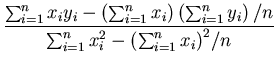
Eq. 4 gives two linear equations in a and b, which can be solved to get
a = 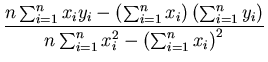 , ,
|
(5) |
with b obtained through subsequent substitution of a in either of the two equations given by
Eq. 4.
In the case of the data given in Figure 1, the best fit line has a slope of 1.64 and intercept
of -0.36. Or in other words,
= 1.64x - 0.36. Note that this is only a best fit line which can be
used to compute the fuel consumption given the weight within or very close to the range of the measurements.
Its predictive power is rather limited. For instance, for x = 0, we get y = - 0.36, which
is non-physical. A physical model for the fuel consumption would have predicted 0 consumption
of fuel for 0 weight.
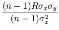
How are the slope and the intercept of the best fit line related to the correlation coefficient?
To examine this, we rewrite Eq. 5 as
| a |
= |
|
|
| |
|
=  |
|
| |
|
= 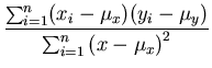 (Verify this step) (Verify this step) |
|
| |
|
=  (See Eq. 1) (See Eq. 1) |
|
| |
|
= R . . |
(6) |
Similarly, from the first of Eq. 4 and the above result we get
so that the equation of the best fit line can be represented by
Next: Tests for the Regression
Up: 10.001: Correlation and Regression
Previous: Correlation Analysis
Michael Zeltkevic
1998-04-15