Subsections
16.5 Steady Quasi-One-Dimensional Heat Flow in Non-Planar Geometry
The quasi one-dimensional equation that has been developed can also
be applied to non-planar geometries, such as cylindrical and
spherical shells.
16.5.1 Cylindrical Shell
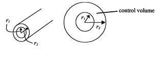
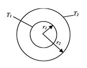
An important case is a cylindrical shell, a geometry often
encountered in situations where fluids are pumped and heat is
transferred. The configuration is shown in
Figure 16.10.
Figure 16.10:
Cylindrical shell geometry notation
|
|
For a steady axisymmetric configuration, the temperature depends
only on a single coordinate ( ) and
Equation (16.13) can be written as
) and
Equation (16.13) can be written as
 |
(16..25) |
or, since
 ,
,
 |
(16..26) |
The steady-flow energy equation (no fluid flow, no work) tells us
that
 , or
, or
 |
(16..27) |
The heat transfer rate per unit length is given by
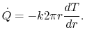 |
(16..28) |
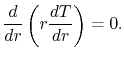
Equation (16.26) is a second order
differential equation for  . Integrating this equation once gives
 |
(16..29) |
where  is a constant of integration.
Equation (16.29) can be written
as
is a constant of integration.
Equation (16.29) can be written
as
 |
(16..30) |
where both sides of
Equation (16.30) are exact
differentials. It is useful to cast this equation in terms of a
dimensionless normalized spatial variable so we can deal with
quantities of order unity. To do this, divide through by the inner
radius,  ,
,
 |
(16..31) |
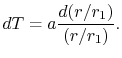
Integrating (16.31) yields
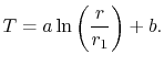 |
(16..32) |
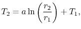
To find the constants of integration
and  , boundary
conditions are needed. These will be taken to be known temperatures
, boundary
conditions are needed. These will be taken to be known temperatures
 and
and  at
and
at
and  respectively. Applying
  at
at  gives
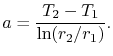
gives  . Applying
  at
at  yields
or
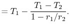
The temperature distribution is thus
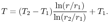 |
(16..33) |
As said, it is generally useful to put expressions such as
(16.33) into non-dimensional and normalized form so that we can deal
with numbers of order unity (this also helps in checking whether
results are consistent). If convenient, having an answer that goes
to zero at one limit is also useful from the perspective of ensuring
the answer makes sense. Equation
(16.33) can be put in
nondimensional form as
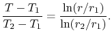 |
(16..34) |
The heat transfer rate,  , is given by
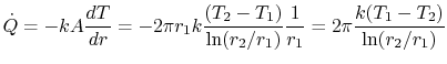 |
(16..35) |
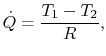
per unit length. When the heat flow rate is written so as to
incorporate our definition of thermal resistance,
comparison with
(16.35) reveals the
thermal resistance  to be
to be
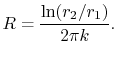 |
(16..36) |
The cylindrical geometry can be viewed as a limiting case of the
planar slab problem. To make the connection, consider the case when
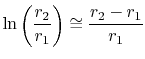
 . From the series expansion for
 we
recall that
we
recall that
 |
(16..37) |
(Look it up, try it numerically, or use the binomial theorem on the
series (
 ) and integrate term by term.)
The logarithms in Equation (16.34)
can thus be written as
 |
(16..38) |
and
 |
(16..39) |
in the limit of
 . Using these expressions in
Equation (16.33) gives
. Using these expressions in
Equation (16.33) gives
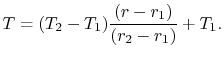 |
(16..40) |
With the substitution of
 , and
, and
 we
obtain
we
obtain
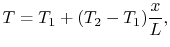 |
(16..41) |
which is the same as Equation (16.19). The
plane slab is thus the limiting case of the cylinder if
, where the heat transfer can be regarded as taking
place in (approximately) a planar slab.
To see when this is appropriate, consider the expansion
 , which is the ratio of heat flux for a cylinder and a
plane slab.
, which is the ratio of heat flux for a cylinder and a
plane slab.
For  error, the ratio of thickness to inner radius should be
less than 0.2, and for 20% error, the thickness to inner radius
should be less than 0.5
(Table 16.2).
error, the ratio of thickness to inner radius should be
less than 0.2, and for 20% error, the thickness to inner radius
should be less than 0.5
(Table 16.2).
Table 16.2:
Utility of plane slab approximation

|
0.1 |
0.2 |
0.3 |
0.4 |
0.5 |

|
0.95 |
0.91 |
0.87 |
0.84 |
0.81 |
|
16.5.2 Spherical Shell
A second example is the spherical shell with specified temperatures
 and
and
 , as sketched in
Figure 16.11.
, as sketched in
Figure 16.11.
Figure 16.11:
Spherical shell
|
|
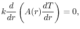
The area is now
 , so the equation for the
temperature field is
, so the equation for the
temperature field is
 |
(16..42) |
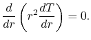
Integrating Equation (16.42) once yields
 |
(16..43) |
Integrating again gives
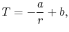 |
(16..44) |
or, normalizing the spatial variable
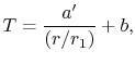 |
(16..45) |
where  and
are constants of integration. As before, we
specify the temperatures at
and
. Use of the
first boundary condition gives
and
are constants of integration. As before, we
specify the temperatures at
and
. Use of the
first boundary condition gives
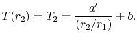
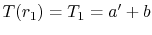 . Applying the
second boundary condition gives
. Applying the
second boundary condition gives
Solving for
and
,
In non-dimensional form the temperature distribution is thus
 |
(16..48) |
UnifiedTP
|