Banner

VII. Production of Thrust with a Propeller

A.   Overview of propeller performance

Each propeller blade is a rotating airfoil which produces lift and drag, and because of a (complex helical) trailing vortex system has an induced upwash and an induced downwash.

Cessna Skyhawk

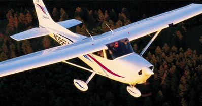
Figure 7.1 Cessna Skyhawk single engine propeller plane (Cessna, 2000)


Schematic of propeller

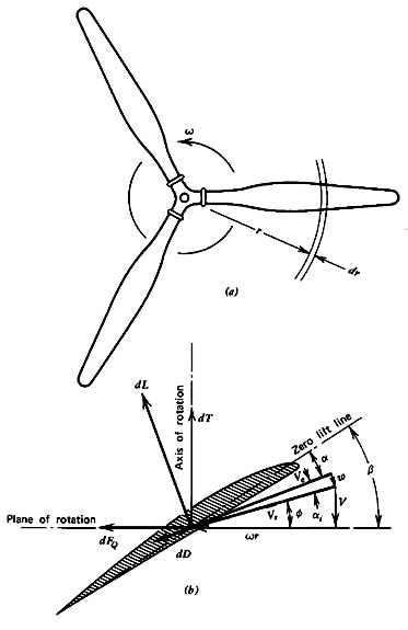
Figure 7.2 Schematic of propeller (McCormick, 1979)


The two quantities of interest are the thrust (T) and the torque (Q).  We can write expressions for these for a small radial element (dr) on one of the blades:


where

                  and      

It is possible to integrate the relationships as a function of r with the appropriate lift and drag coefficients for the local airfoil shape, but determining the induced upwash (ai) is difficult because of the complex helical nature of the trailing vortex system.  In order to learn about the details of propeller design, it is necessary to do this.  However, for our purposes, we can learn a about the overall performance features using the integral momentum theorem, some further approximations called “actuator disk theory”, and dimensional analysis.


NASA Glenn has a nice explanation of propeller thrust - GO!


V-22

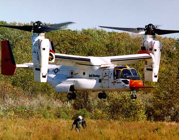
Figure 7.3 The V-22 Osprey utilizes tiltrotor technology (Boeing, 2000)


B.   Application of the Integral Momentum Theorem to Propellers

Control Volume for Analysis of a Propeller    for analysis of a propeller

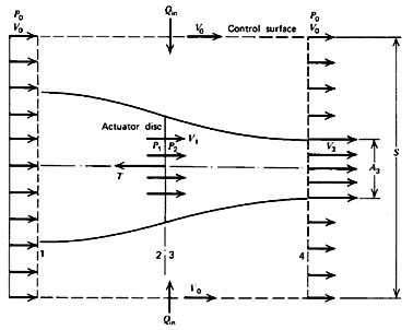
Figure 7.4 Control volume for analysis of a propeller (McCormick, 1979)


The control volume shown in Figure 7.3 has been drawn far enough from the device so that the pressure is everywhere equal to a constant.  This is not required, but it makes it more convenient to apply the integral momentum theorem.  We will also assume that the flow outside of the propeller streamtube does not have any change in total pressure.  Then since the flow is steady we apply:


Since the pressure forces everywhere are balanced, then the only force on the control volume is due to the change in momentum flux across its boundaries.  Thus by inspection, we can say that


Or we can arrive at the same result in a step-by-step manner as we did for the jet engine example in Section II:


Note that the last term is identically equal to zero by conservation of mass.  If the mass flow in and out of the propeller streamtube are the same (as we have defined), then the net mass flux into the rest of the control volume must also be zero.

So we have:


as we reasoned before.

The power expended is equal to the power imparted to the fluid which is the change in kinetic energy of the flow as it passes through the propeller


The propulsive power is the rate at which useful work is done which is the thrust multiplied by the flight velocity


The propulsive efficiency is then the ratio of these two:


Which is the same expression as we arrived at before for the jet engine (as you might have expected).


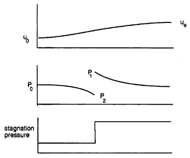
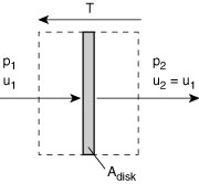
C.   Actuator Disk Theory

To understand more about the performance of propellers, and to relate this performance to simple design parameters, we will apply actuator disk theory.  We model the flow through the propeller as shown in Figure 7.4 and make the following assumptions:

Actuator Disk Model

Figure 7.5 Schematic of actuator disk model (Kerrebrock).


We then take a control volume around the disk as shown in Figure 7.5

Actuator Disk

Figure 7.6 Control volume around actuator disk.


The force, T,  on the disk is


So the power is


We also know that the power is


Thus we see that the velocity at the disk is


Half of the axial velocity change occurs upstream of the disk and half occurs downstream of the disk.

We can now find the pressure upstream and downstream of the disk by applying the Bernoulli equation in the regions of the flow where the pressure and velocity are varying continuously.

                           and                  

From which we can determine


We generally don’t measure or control udisk directly.  Therefore, it is more useful to write our expressions in terms of flight velocity uo, thrust, T, (which must equal drag for steady level flight) and propeller disk area, Adisk.


So


From which we can obtain an expression for the exit velocity in terms of thrust and flight velocity which are vehicle parameters


The other parameters of interest become


This is the ideal (minimum) power required to drive the propeller.  In general , the actual power required would be about 15% greater than this.


There are several important trends that are apparent upon consideration of these equations.  We see that the propulsive efficiency is zero when the flight velocity is zero (no useful work, just a force), and tends towards one when the flight velocity increases.  In practice, the propulsive efficiency typically peaks at a level of around 0.8 for a propeller before various aerodynamic effects act to decay its performance as will be shown in the following section.


D. Dimensional Analysis

We will now use dimensional analysis to arrive at a few important parameters for the design and choice of a propeller.  Dimensional analysis leads to a number of coefficients which are useful for presenting performance data for propellers.

Parameter

Symbol

Units

propeller diameter

D

m

propeller speed

n

rev/s

torque

Q

Nm

thrust

T

N

fluid density

r

kg/m3

fluid viscosity

n

m2/s

fluid bulk elasticity modulus

K

N/m2

flight velocity

uo

m/s

1.     Thrust Coefficient

            T = f(D; n; r; n; K; uo) = Const. Da nb rc nd Ke uof

      Then putting this in dimensional form

            [MLT-2] = [(L)a(T)-b(ML-3)c(L2T-1)d(ML-1T-2)e(LT-1)f]

      Which implies

(M)            1= c+ e

(L)               1 = a - 3c + 2d ­ e + f

(T)         2 = b + d + 2e + f

      So

            a = 4 ­ 2e ­ 2d ­ f

            b = 2 ­ d ­ 2e ­ f

            c = 1 - e

            T = Const. D4-2e-2d-f n2-d-2e-f r1-e nd Ke uof


      We can now consider the three terms in the square brackets

      : Dn is proportional to the tip speed, so this term is like

      : K/r = a2 where a is the speed of sound, this is like

      : uo/n is the distance advanced by the propeller in one revolution, here non-dimensionalized by the propeller diameter.

      This last coefficient is typically called the advance ratio and given the symbol J.

      Thus we see that the thrust may be written as


      which is often expressed as

                                                 where kT is called the thrust coefficient and in general is a function of propeller design, Re, Mtip and J.

2.  Torque Coefficient

We can follow the same steps to arrive at a relevant expression and functional dependence for the torque or apply physical reasoning.  Since torque is a force multiplied by a length, it follows that

                                                 where kQ is called the thrust coefficient and in general is a function of propeller design, Re, Mtip and J.

3.     Efficiency

The power supplied to the propeller is Pin where


The useful power output is Pout where


Therefore the efficiency is given by


4.     Power Coefficient

The power required to drive the propeller is


which is often written using a power coefficient Cp = 2pkQ

                                            then                                            


E. Typical propeller performance

Typical propeller performance curves are shown in the following figures.

propeller efficiency curves

Figure 7.7 Typical propeller efficiency curves as a function of advance ratio (J=uo/nD) and blade angle(McCormick, 1979).


propeller thrust curves

Figure 7.8 Typical propeller thrust curves as a function of advance ratio (J=uo/nD) and blade angle (McCormick, 1979).


propeller power curves

Figure 7.9 Typical propeller power curves as a function of advance ratio (J=uo/nD) and blade angle (McCormick, 1979).


<< Previous Unified Propulsion Next >>