Subsections
As with all sciences, thermodynamics is concerned with the
mathematical modeling of the real world. In order that the
mathematical deductions are consistent, we need some precise
definitions of the basic concepts. The following is a discussion of
some of the concepts we will need. Several of these will be further
amplified in the lectures and in other handouts. If you need
additional information or examples concerning these topics, they are
described clearly and in-depth in (SB&VW). They are also covered,
although in a less detailed manner, in Chapters 1 and 2 of the book
by Van Ness.
Matter may be described at a molecular (or microscopic) level using
the techniques of statistical mechanics and kinetic theory. For
engineering purposes, however, we want ``averaged'' information,
i.e., a macroscopic, not a microscopic, description. There are two
reasons for this. First, a microscopic description of an engineering
device may produce too much information to manage. For example,
 of air at standard temperature and pressure
contains
of air at standard temperature and pressure
contains  molecules (VW, S & B:2.2), each of which has a
position and a velocity. Typical engineering applications involve
more than
molecules (VW, S & B:2.2), each of which has a
position and a velocity. Typical engineering applications involve
more than  molecules. Second, and more importantly,
microscopic positions and velocities are generally not useful for
determining how macroscopic systems will act or react unless, for
instance, their total effect is integrated. We therefore neglect the
fact that real substances are composed of discrete molecules and
model matter from the start as a smoothed-out
continuum. The information we have about a
continuum represents the microscopic information averaged over a
volume. Classical thermodynamics is concerned only with
continua.
molecules. Second, and more importantly,
microscopic positions and velocities are generally not useful for
determining how macroscopic systems will act or react unless, for
instance, their total effect is integrated. We therefore neglect the
fact that real substances are composed of discrete molecules and
model matter from the start as a smoothed-out
continuum. The information we have about a
continuum represents the microscopic information averaged over a
volume. Classical thermodynamics is concerned only with
continua.
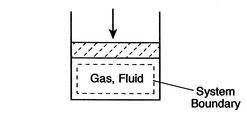
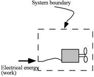
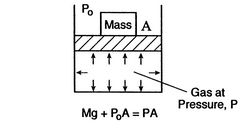
A thermodynamic system is a quantity of matter of fixed
identity, around which we can draw a boundary (see
Figure 1.3 for an example). The
boundaries may be fixed or moveable. Work or heat can be
transferred across the system boundary. Everything outside the
boundary is the surroundings.
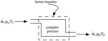
When working with devices such as engines it is often useful to
define the system to be an identifiable volume with flow in
and out. This is termed a control volume. An example is
shown in Figure 1.5.
A closed system is a special class of
system with boundaries that matter cannot cross. Hence the
principle of the conservation of mass is automatically satisfied
whenever we employ a closed system analysis. This type of system is
sometimes termed a control mass.
Figure 1.3:
Piston (boundary) and gas (system)
|
|
Figure 1.4:
Boundary around electric motor (system)
|
|
Figure 1.5:
Sample control volume
|
|
1.2.3 The Concept of a ``State''
The thermodynamic state
of a
system is defined by specifying values of a set of measurable
properties sufficient to determine all other properties.
For fluid systems, typical properties are pressure, volume and
temperature. More complex systems may require the specification of
more unusual properties. As an example, the state of an electric
battery requires the specification of the amount of electric charge
it contains.
Properties may be extensive or intensive.
Extensive properties are additive. Thus, if the system is divided
into a number of sub-systems, the value of the property for the
whole system is equal to the sum of the values for the parts.
Volume is an extensive property. Intensive properties do not
depend on the quantity of matter present. Temperature and
pressure are intensive properties.
Specific properties are
extensive properties per unit mass and are denoted by lower case
letters. For example:
Specific properties are intensive because they do not depend on the
mass of the system.
The properties of a simple system are uniform throughout.
In general, however, the properties of a system can vary from point
to point. We can usually analyze a general system by sub-dividing it
(either conceptually or in practice) into a number of simple systems
in each of which the properties are assumed to be uniform.
It is important to note that properties describe states only
when the system is in equilibrium.
Muddy Points
Specific properties (MP 1.1)
What is the difference between extensive and intensive properties?
(MP 1.2)
The state of a system in
which properties have definite, unchanged values as long as external
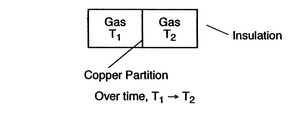
conditions are unchanged is called an equilibrium state.
Figure 1.6:
Equilibrium
[Mechanical Equilibrium]
[Thermal Equilibrium]
|
A system in thermodynamic equilibrium satisfies:
- mechanical equilibrium (no unbalanced forces)
- thermal equilibrium (no temperature differences)
- chemical equilibrium.
If the state of a system changes, then it is undergoing a
process. The succession of states
through which the system passes defines the path of the
process. If, at the end of the process, the properties
have returned to their original values, the system has undergone a
cyclic process or a cycle.
Note that even if a system has returned to its original state and
completed a cycle, the state of the surroundings may have changed.
We are often interested in charting thermodynamic processes between
states on thermodynamic coordinates. Recall from the end of
Section 1.2.3, however, that properties define a state
only when a system is in equilibrium. If a process involves finite,
unbalanced forces, the system can pass through non-equilibrium
states, which we cannot treat. An extremely useful idealization,
however, is that only ``infinitesimal'' unbalanced forces exist, so
that the process can be viewed as taking place in a series of
``quasi-equilibrium'' states. (The term quasi can be taken to
mean ``as if;'' you will see it used in a number of contexts such as
quasi-one-dimensional, quasi-steady, etc.) For this to be true the
process must be slow in relation to the time needed for the system
to come to equilibrium internally. For a gas at conditions of
interest to us, a given molecule can undergo roughly  molecular collisions per second, so that, if ten collisions are
needed to come to equilibrium, the equilibration time is on the
order of
molecular collisions per second, so that, if ten collisions are
needed to come to equilibrium, the equilibration time is on the
order of  seconds. This is generally much shorter than the
time scales associated with the bulk properties of the flow (say the
time needed for a fluid particle to move some significant fraction
of the length of the device of interest). Over a large range of
parameters, therefore, it is a very good approximation to view the
thermodynamic processes as consisting of such a succession of
equilibrium states, which we can chart. [VW, S& B: 2.3-2.4]
seconds. This is generally much shorter than the
time scales associated with the bulk properties of the flow (say the
time needed for a fluid particle to move some significant fraction
of the length of the device of interest). Over a large range of
parameters, therefore, it is a very good approximation to view the
thermodynamic processes as consisting of such a succession of
equilibrium states, which we can chart. [VW, S& B: 2.3-2.4]
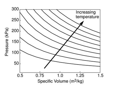
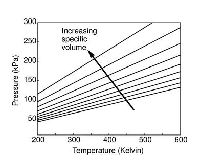
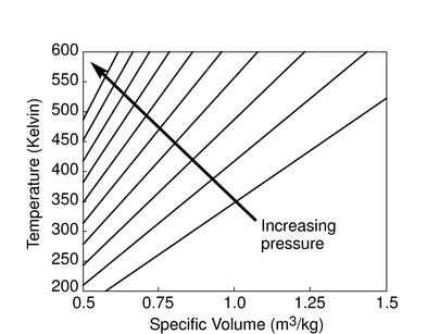
The figures below demonstrate the use of thermodynamics coordinates
to plot isolines, lines along which a property is constant. They
include constant temperature lines, or isotherms, on a
 -
- diagram, constant volume lines, or isochors on a
 -
diagram, and constant pressure lines, or isobars,
on a
-
diagram for an ideal gas.
-
diagram, and constant pressure lines, or isobars,
on a
-
diagram for an ideal gas.
Real substances may have phase changes (water to water vapor, or
water to ice, for example), which we can also plot on thermodynamic
coordinates. We will see such phase changes plotted and used for
liquid-vapor power generation cycles in Chapter 8. A
preview is given in Figure 1.15 at the end of
this chapter.
Figure:
-
diagram
Figure:
-
diagram
Figure:
-
diagram
Figure 1.7:
Thermodynamics coordinates and isolines for an ideal gas
|
|
It is an experimental fact that two properties are needed to define
the state of any pure substance in equilibrium or undergoing a
steady or quasi-steady process. [VW, S & B: 3.1, 3.3].
Thus for a simple compressible
gas like air,
where
is the volume per unit mass,  . In words, if we
know
and
we know
. In words, if we
know
and
we know  , etc.
Any of these is equivalent to an equation
 , which is
known as an equation of state. The equation of state for an ideal
gas, which is a very good approximation to real gases at conditions
that are typically of interest for aerospace
applications1.2, is
, which is
known as an equation of state. The equation of state for an ideal
gas, which is a very good approximation to real gases at conditions
that are typically of interest for aerospace
applications1.2, is
where  is the volume per mol of gas and
 is
the ``Universal Gas Constant,''
is
the ``Universal Gas Constant,''
 .
.
A form of this equation which is more useful in fluid flow problems
is obtained if we divide by the molecular weight,
 :
:
where R is
 , which has a different value
for different gases due to the different molecular weights. For air
at room conditions,
, which has a different value
for different gases due to the different molecular weights. For air
at room conditions,
 .
.
Douglas Quattrochi
2006-08-06
|