11.10
Summary

Far reaching as they are, the laws summarized by Maxwell's equations are directly applicable to the description of only one of many physical subsystems of scientific and engineering interest. Like those before it, this chapter has been concerned with the electromagnetic subsystem. However, by casting the electromagnetic laws into statements of power flow, we have come to recognize how the electromagnetic subsystem couples to the thermodynamic subsystem through the power dissipation density and to the mechanical subsystem through forces and force densities of electromagnetic origin.

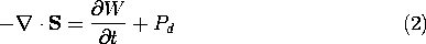
The basis for a self-consistent macroscopic description of any continuum subsystem is a power flow statement having the forms identified in Sec. 11.1. Describing the energy and power flow in and into a volume V enclosed by a surface S, the integral conservation of energy statement takes the form (11.1.1).

The differential form of the conservation of energy statement is implied by the above.

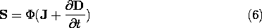
Poynting's theorem, the subject of Sec. 11.2, is obtained starting from the laws of Faraday and Ampère to obtain an expression of the form of (2). For materials that are Ohmic (J = E) and that are linearly polarizable and magnetizable (D = E and B = H), the power flux density S (or Poynting's vector), energy density W, and power dissipation density P_d were shown in Sec. 11.3 to be

Of course, taking the free space limit where and assume their free space values and = 0 gives the free space conservation statement discussed in Sec. 11.2.

In Sec. 11.3, we found that in EQS systems, an alternative to Poynting's vector is (11.3.24).

This expression is of practical importance, because it can be evaluated without determining H, which is generally not of interest in EQS systems.

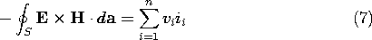
An important application of the integral form of the energy conservation statement is to lumped parameter systems. In these cases, the surface S of (1) encloses a system that is connected to the outside world through terminals. It is then convenient to describe the power flow in terms of the terminal variables. It was shown in Sec. 11.3 (11.3.29), that the net power into the system represented by the left-hand side of (1) becomes

provided that the magnetic induction and the electric displacement current through the surface S are negligible.

This set the stage for the application of the integral form of the energy conservation theorem to lumped parameter systems.

In Sec. 11.4, attention focused on the energy storage term, the first terms on the right in (1) and (2). The energy density concept was broadened to include materials having constitutive laws relating the flux densities to the field intensities that were single valued and collinear. With E, D, H, and B representing the field magnitudes, the energy density was found to be the sum of electric and magnetic energy densities.

Integrated over the volume V of a system, this function leads to the total energy w.

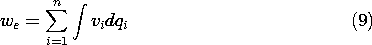
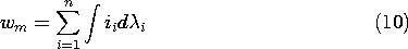
For quasistatic lumped parameter systems, the total electric or magnetic energy is often conveniently found following a different route. First the terminal relations are determined and then the total energy is found by adding up the increments of energy put into the system as it is energized. In the case of an n terminal pair EQS system, where the relation between terminal voltage v_i and associated charge q_i is v_i (q₁, q₂, q_n ), the increment of energy is v_i dq_i, and the total electric energy is (11.4.9).

The line integration in an n-dimensional space representing the n independent q_i's was illustrated by Example 11.4.2.

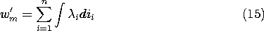
Similarly, for an n terminal pair MQS system where the current i_i is related to the flux linkage _i by i_i = i_i (₁, ₂, _n), the total energy is (11.4.12).

Note the analogy between these expressions for the total energy of EQS and MQS lumped parameter systems and the electric and magnetic energy densities, respectively, of (8). The transition from the field picture afforded by the energy densities to the lumped parameter characterization is made by E v, D q and by H i, B .

Especially in using the energy to evaluate forces of electrical origin, we found it convenient to define coenergy density functions.

It followed that these functions were natural when it was desirable to use E and H as the independent variables rather than D and B.

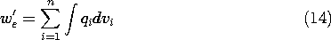
The total coenergy functions for lumped parameter EQS and MQS systems could be found either by integrating these densities over the volume or by again viewing the system in terms of its terminal variables. With the total coenergy functions defined by

it followed that the coenergy functions could be determined from the terminal relations by again carrying out line integrations, but this time with the voltages and currents as the independent variables. For EQS systems,

while for MQS systems,

Again, note the analogy to the respective terms in (12).

The remaining sections of the chapter developed some of the possible implications of the "dissipation" term in the energy conservation statement, the last terms in (1) and (2). In Sec. 11.5, coupling to a thermal subsystem was discussed. In this section, the disparity between the power input and the rate of increase of the energy stored was accounted for by heating. In addition to Ohmic heating, caused by collisions between the migrating carriers and the neutral media, we considered losses associated with the dynamic polarization and magnetization of materials.

In Secs. 11.6-11.9, we considered coupling to a mechanical subsystem as a second mechanism by which energy could be extracted from (or put into) the electromagnetic subsystem. With the displacement of an object denoted by , we used an energy conservation postulate to infer the total electric or magnetic force acting on the object from the energy functions [(11.6.9), and its magnetic analog]

or from the coenergy functions [(11.7.7) and the analogous expression for electric systems].

In Sec. 11.8, where the Lorentz force on a particle was generalized to account for electric and magnetic dipole moments, one objective was a microscopic picture that would lend physical insight into the forces on polarized and magnetized materials. The Lorentz force was generalized to include the force on stationary electric and magnetic dipoles, respectively.

The total macroscopic forces resulting from microscopic forces had already been encountered in the previous two sections. The force density describes the interaction between a volume element of the electromagnetic subsystem and a mechanical continuum. The force density inferred by averaging over the forces identified in Sec. 11.8 as acting on microscopic particles was

A more rigorous approach to finding the force density could be based on a generalization of the energy method introduced in Secs. 11.6 and 11.7. As background for further pursuit of this subject, we have illustrated the importance of including the mechanical continuum with which the force density acts. Before there can be a meaningful answer to the question, "Which force density is correct?" the other force densities acting on the material must be specified. As an illustration, we found that very different electric or magnetic force densities would result in the same deformations of an incompressible material and in the same net force on an object surrounded by free space^[1,2].