14.5
Transmission Lines in the Sinusoidal Steady State

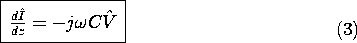
The method used in Sec. 14.4 is equally applicable to finding the response to a sinusoidal excitation of an ideal transmission line. Rather than exciting the line by a voltage step or a voltage pulse, as in the examples of Sec. 14.4, the source may produce a sinusoidal excitation. In that case, there is a part of the response that is in the sinusoidal steady state and a part that accounts for the initial conditions and the transient associated with turning on the source. Provided that the boundary conditions are (like the transmission line equations) linear, we can express the response as a superposition of these two parts.

Here, V_s is the sinusoidal steady state response, determined without regard for the initial conditions but satisfying the boundary conditions. Added to this to make the total solution satisfy the initial conditions is V_t. This transient solution is defined to satisfy the boundary conditions with the drive equal to zero and to make the total solution satisfy the initial conditions. If we were interested in it, this transient solution could be found using the methods of the previous section. In an actual physical situation, this part of the solution is usually dissipated in the resistances of the terminations and the line itself. Then the sinusoidal steady state prevails. In this and the next section, we focus on this part of the solution.

With the understanding that the boundary conditions, like those describing the transmission line, are linear differential equations with constant coefficients, the response will be sinusoidal and at the same frequency, , as the drive. Thus, we assume at the outset that

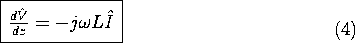
Substitution of these expressions into the transmission line equations, (14.1.4)-(14.1.5), shows that the z dependence is governed by the ordinary differential equations

Again because of the constant coefficients, these linear equations have two solutions, each having the form exp (-jkz). Substitution shows that

where LC. In terms of the same two arbitrary complex coefficients, it also follows from substitution of this expression into (14.1.5) that

where Z_o = L/C.

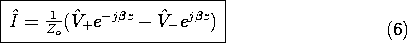
What we have found are solutions having the same traveling wave forms as identified in Sec. 14.3, (14.3.9)-(14.3.10). This can be seen by using (2) to recover the time dependence and writing these two expressions as

The velocity of the waves is / = 1/LC. Because the coefficients are complex, they represent both the amplitude and phase of these traveling waves. Thus, the solutions could be sinusoids, cosinusoids, or any combination of these having the given arguments. In working with standing waves in Sec. 13.2, we demonstrated how the coefficients could be adjusted to satisfy simple boundary conditions. Here we introduce a point of view that is convenient in dealing with complicated terminations.

Transmission Line Impedance

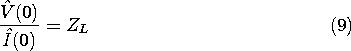
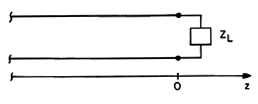
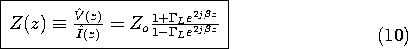
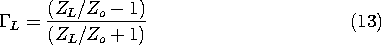
The transmission line shown in Fig. 14.5.1 is terminated in a load impedance Z_L. By definition, Z_L is the complex number

Fig 14.5.1 Termination at z = 0 in load impedance.

In general, it could represent any linear system composed of resistors, inductors, and capacitors. The complex amplitudes are determined by this and another boundary condition. This second condition represents the termination of the line somewhere to the left in Fig. 14.5.1.

At any location on the line, the impedance is found by taking the ratio of (5) and (6).

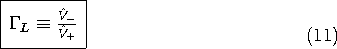
Here, _L is the reflection coefficient of the load.

Thus, _L is simply the ratio of the complex amplitudes of the traveling wave components.

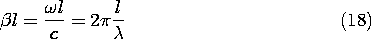
At the location z = 0, where the line is connected to the load and (9) applies, this expression becomes

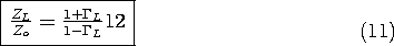
The boundary condition, expressed by (12), is sufficient to determine the reflection coefficient. That is, from (12) it follows that

Given the load impedance, _L follows from this expression. The line impedance at a location z to the left then follows from the use of this expression to evaluate (10).

The following examples lead to important implications of (11) while indicating the usefulness of the impedance point of view.

Example 14.5.1. Impedance Matching

Given an incident wave V₊, how can we eliminate the reflected wave represented by V_-? By definition, there is no reflected wave if the reflection coefficient, (11), is zero. It follows from (13) that

Note that Z_o is real, which means that the matched load is equivalent to a resistance, R_L = Z_o. Thus, our finding is consistent with that of Sec. 14.4, where we found that such a termination would eliminate the reflected wave, sinusoidal steady state or not.

It follows from (10) that the line has the same impedance, Z_o, at any location z, when terminated in its characteristic impedance. Because V_-=0, it follows from (7) that the voltage takes the form

The voltage has the distribution in space and time of a sinusoid traveling in the z direction with the velocity 1/LC. At any given location, the voltage is sinusoidal in time at the (angular) frequency . The amplitude is the same, regardless of z.

---

⁶ By contrast with Demonstration 13.1.1, where the light emitted by the fluorescent tube indicated that the electric field peaked at some locations and nulled at others, the distribution of light for a matched line would be "flat."

---

The previous example illustrated that at any location, a transmission line terminated in a resistance equal to its characteristic impedance has an impedance which is also resistive and equal to Z_o. The next example illustrates what happens in the opposite extreme, where the termination dissipates no energy and the response is a pure standing wave rather than the pure traveling wave of the matched line.

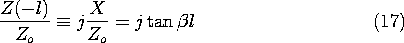
Example 14.5.2. Short Circuit Impedance and Standing Waves

With a short circuit at z = 0, (5) makes it clear that V_- = -V₊. Thus, the reflection coefficient defined by (11) is _L = -1. We come to the same conclusion from the evaluation of (13).

The impedance at some location z then follows from (10) as

In view of the definition of ,

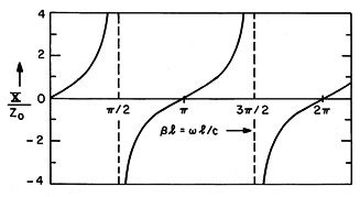
and so we can think of l as being proportional either to the frequency or to the length of the line measured in wavelengths . The impedance of the line is a reactance X having the dependence on either of these quantities shown in Fig. 14.5.2.

Fig 14.5.2 Reactance as a function of normalized frequency for a shorted line.

At low frequencies (or for a length that is short compared to a quarter-wavelength), X is positive and proportional to . As should be expected from either Chap. 8 or Example 13.1.1, the reactance is that of an inductor.

As the frequency is raised to the point where the line is a quarter-wavelength long, the impedance is infinite. A shorted quarter-wavelength line has the impedance of an open circuit! As the frequency is raised still further, the reactance becomes capacitive, decreasing with increasing frequency until the half-wavelength line exhibits the impedance of the termination, a short. That the impedance repeats itself as the line is increased in length by a half-wavelength is evident from Fig. 14.5.2.

We consider next an example that illustrates one of many methods for matching a load resistance R_L to a line having a characteristic impedance not equal to R_L.

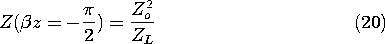
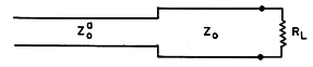
Example 14.5.3. Quarter-Wave Matching Section

A quarter-wavelength line, as shown in Fig. 14.5.3, has the useful property of converting a normalized load impedance Z_L/Z_o to a normalized impedance that is the reciprocal of that impedance, Z_o/Z_L. To see this, we evaluate the impedance, (10), a quarter-wavelength from the load, where z = - /2, and then use (12).

Fig 14.5.3 A quarter-wave matching section.

Thus, if we wanted to match a line having the characteristic impedance Z^a_o to a load resistance Z_L = R_L, we could interpose a quarter-wavelength section of line having as its characteristic impedance a Z_o that is the geometric mean of the load resistance and the characteristic impedance of the line to be matched.

The idea of using quarter-wavelength sections to achieve matching will be continued in the next example.

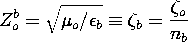
The transmission line model is equally well applicable to electromagnetic plane waves. The equivalence was pointed out in Sec. 14.1. When these waves are optical, the permeability of common materials remains _o, and the polarizability is described by the index of refraction, n, defined such that

Thus, n² _o takes the place of the dielectric constant, . The appropriate value of n² _o is likely to be very different from the value of used for the same material at low frequencies.

⁷ With fields described in the frequency domain, , and hence n², are in general complex functions of frequency, as in Sec. 11.5.

The following example illustrates the application of the transmission line viewpoint to an optical problem.

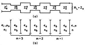
Example 14.5.4. Quarter-Wave Cascades for Reduction of Reflection

When one quarter-wavelength line is used to transform from one specified impedance to another, it is necessary to specify the characteristic impedance of the quarter-wave section. In optics, where it is desirable to minimize reflections that result from the passage of light from one transparent medium to another, it is necessary to specify the index of refraction of the quarter wave section. Given other constraints on the materials, this often is not possible. In this example, we see how the use of multiple layers gives some flexibility in the choice of materials.

The matching section of Fig. 14.5.4a consists of m pairs of quarter-wave sections of transmission line, respectively, having characteristic impedances Z_o^a and Z_o^b. This represents equally well the cascaded pairs of quarter wave layers of dielectric shown in Fig. 14.5.4b, interposed between materials of dielectric constants and _i. Alternatively, these layers are represented by their indices of refraction, n_a and n_b, interposed between materials having indices n_i and n.

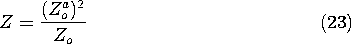
Fig 14.5.4 (a) Cascaded quarter-wave transmission line sections. (b) Optical coating represented by (a).

First, we picture the matching problem in terms of the transmission line. The load resistance R_L represents the material to the right of the cascade. This region is pictured as an infinite transmission line having characteristic impedance Z_o. Thus, it presents a load to the cascade of resistance R_L = Z_o. To determine the impedance at the other side of the cascade, we make repeated use of the impedance transformation for a quarter-wave section, (20). To begin with, the impedance at the terminals of the first quarter-wave section is

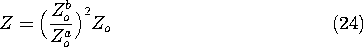
With this taken as the load resistance in (20), the impedance at the terminals of the second section is

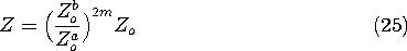
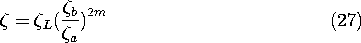
This can now be regarded as the impedance transformation for the pair of quarter-wave sections. If we now make repeated use of (24) to represent the impedance transformation for the quarter-wave sections taken in pairs, we find that the impedance at the terminals of m pairs is

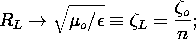
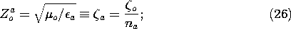
Now, to apply this result to the optics configuration, we identify (14.1.9)

and have from (25) for the intrinsic impedance of the cascade

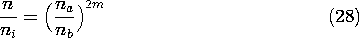
In terms of the indices of refraction,

If this condition on the optical properties and number of the layer pairs is fulfilled, the wave can propagate through the interface between regions of indices n_i and n without reflection. Given materials having n_a/n_b less than n/n_i, it is possible to pick the number of layer pairs, m, to satisfy the condition (at least approximately).

Coatings are commonly used on lenses to prevent reflection. In such applications, the waves processed by the lens generally have a spectrum of frequencies. Thus, optimization of the matching coatings is more complex than pictured here, where it has been assumed that the light is at a single frequency (is monochromatic).

It has been assumed here that the electromagnetic wave has normal incidence at the dielectric interface. Waves arriving at the interface at an angle can also be pictured in terms of the transmission line. In practical applications, the design of lens coatings to prevent reflection over a range of angles of incidence is a further complication.

---

⁸ H. A. Haus, Waves and Fields in Optoelectronics, Prentice-Hall, Inc., Englewood Cliffs, N.J. (1984), pp. 43-46.

---