Basic Plotting

Table of Contents, Get code for this tutorial

Note: You can execute the code from this tutorial by highlighting them, right-clicking, and selecting "Evaluate Selection" (or hit F9).

In this section, you'll learn about various plotting functions available in MATLAB and how to learn about these commands.

Plot Types
The PLOT function
Titles, Labels, Legends
3D Plots
Customizing Surface Plots
Views
Colormaps
Shading
Lighting
Transparency

Plot Types

MATLAB provides a variety of plotting routines, both in 2D and 3D. Here's a good summary of these plotting routines.

To learn how to use these functions, use help or doc

help scatter
% doc scatter

 SCATTER Scatter/bubble plot.
    SCATTER(X,Y,S,C) displays colored circles at the locations specified
    by the vectors X and Y (which must be the same size).  
 
    S determines the area of each marker (in points^2). S can be a
    vector the same length a X and Y or a scalar. If S is a scalar, 
    MATLAB draws all the markers the same size. If S is empty, the
    default size is used.
    
    C determines the colors of the markers. When C is a vector the
    same length as X and Y, the values in C are linearly mapped
    to the colors in the current colormap. When C is a 
    length(X)-by-3 matrix, it directly specifies the colors of the  
    markers as RGB values. C can also be a color string. See ColorSpec.
 
    SCATTER(X,Y) draws the markers in the default size and color.
    SCATTER(X,Y,S) draws the markers at the specified sizes (S)
    with a single color. This type of graph is also known as
    a bubble plot.
    SCATTER(...,M) uses the marker M instead of 'o'.
    SCATTER(...,'filled') fills the markers.
 
    SCATTER(AX,...) plots into AX instead of GCA.
 
    H = SCATTER(...) returns handles to the scatter objects created.
 
    Use PLOT for single color, single marker size scatter plots.
 
    Example
      load seamount
      scatter(x,y,5,z)
 
    See also SCATTER3, PLOT, PLOTMATRIX.

    Reference page in Help browser
       doc scatter

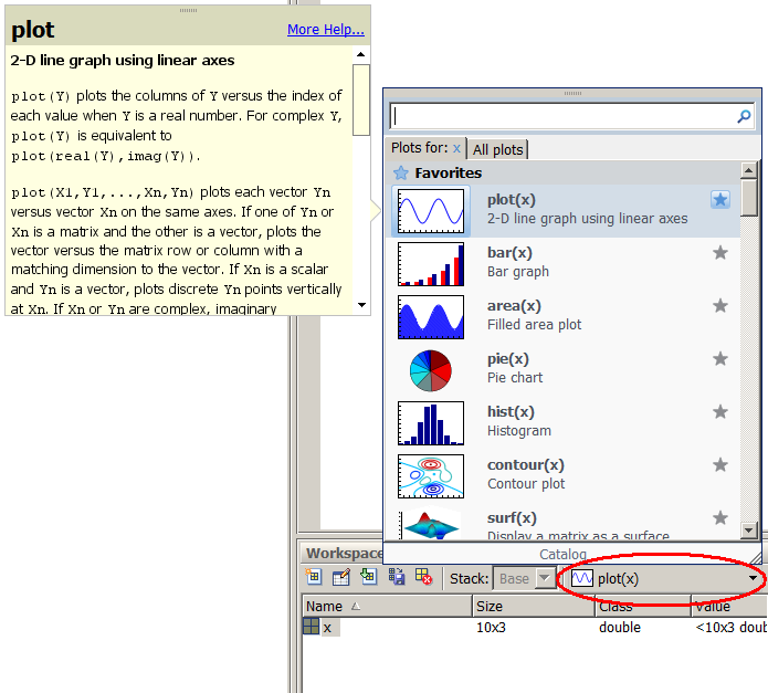
You can also access these functions directly from the Workspace Browser. Just highlight a variable that you want to plot and click on the drop down menu to bring up the Plot Selector.

The PLOT function

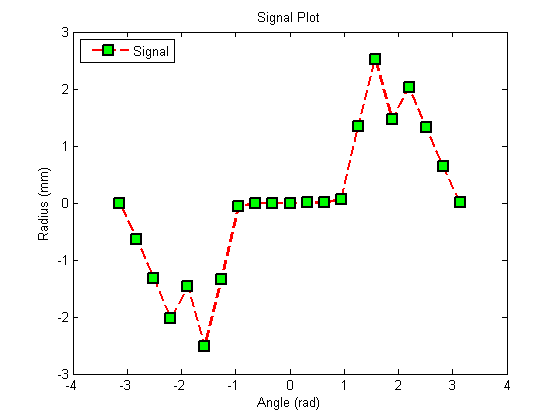
As with many other MATLAB functions, plot takes additional arguments allowing you to customize the plot.

x = -pi:pi/10:pi;
y = tan(sin(x)) - sin(tan(x));
plot(x, y, '--rs');

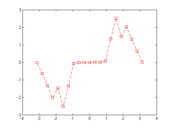
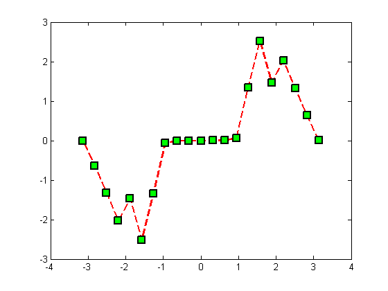
In fact, you have much more control by providing specific "properties" to the command. In the next section, we'll talk more about these properties.

plot(x, y, '--rs', ...
   'LineWidth', 2, ...
   'MarkerEdgeColor', 'k', ...
   'MarkerFaceColor', 'g', ...
   'MarkerSize', 10);

Titles, Labels, Legends

Adding titles, labels, legends is as simple as using the commands title, xlabel, ylabel, legend.

xlabel('Angle (rad)');
ylabel('Radius (mm)');
title('Signal Plot');
legend('Signal', 'Location', 'Northwest');

3D Plots

MATLAB's 3D plotting capability is just as versatile as the 2D plots. Let's first focus on the three different types of 3D plots:

Line plots - these are typically used to plot x, y, z vectors of coordinates.
Patches - these are used to draw 2- or 3-D polygons of arbitrary shape.
Surface plots - these are typically used to plot matrix data.

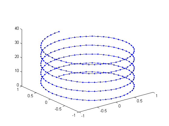
Line Plots

plot3 will plot a 3D line plot connecting consecutive (x, y, z) coordinates.

t = 0:pi/25:10*pi;
x = sin(t); y = cos(t);
plot3(x, y, t, '.-');

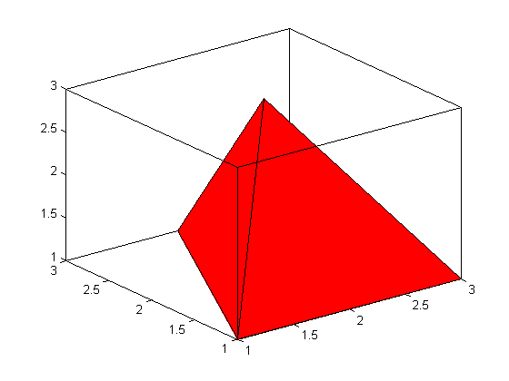
Patches

patch allows you to plot arbitrary shapes by providing coordinates of the patch faces.

clf;
% Plane 1   2   3   4
x =    [1   1   3   2;
        3   3   2   1;
        2   2   2   2];
y =    [1   1   1   3;
        1   1   3   1;
        3   2   2   2];
z =    [1   1   1   1;
        1   1   1   1;
        1   3   3   3];
patch(x, y, z, 'red')
view(3);
box on;

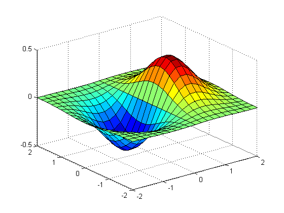
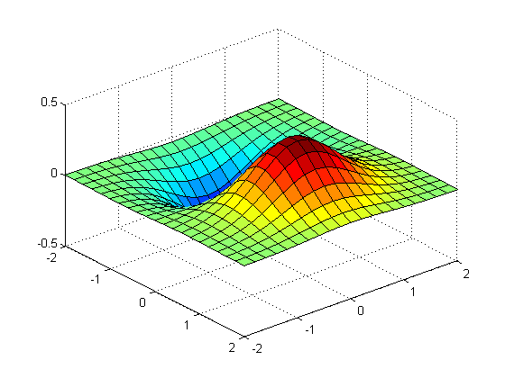
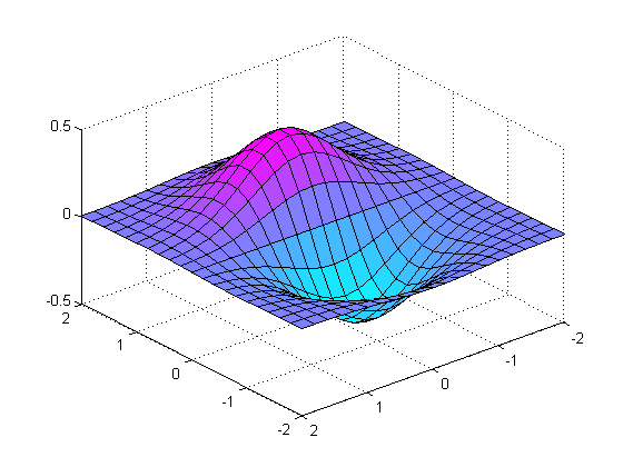
Surface Plots

surf, mesh (and others) require the data to be in a matrix (grid) format. The values of the matrix elements represent the z values in the surface.

X = -2:.2:2;
Y = -2:.2:2;
Z = bsxfun(@(x,y) x.*exp(-x.^2 - y.^2), X, Y');
surf(X, Y', Z);

Customizing Surface Plots

Let's take a look at some behaviors which are common to (but not limited to) surface plots:

Views
Colormaps
Shading
Lighting
Transparency

For the rest of the tutorial, we'll take a look at each of these topics in detail.

Views

In a 3D plot, you can change the orientation of the view. You can do it interactively from the figure window:

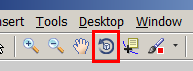
But you can also do it programmatically using the view command.

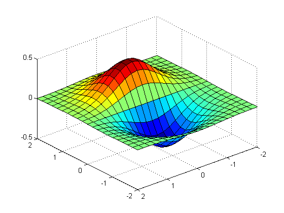
view(50, 40);   % azimuth and elevation

Another way of changing the view is to use commands like camorbit.

camorbit(180, 0);    % 180 degrees about Z-axis

In fact, there are a number of cam* commands for manipulating the view camera. Read more about it here.

Colormaps

Colormaps are MATLAB's way of mapping levels/intensities/values to colors. It exists in all MATLAB graphics, but you see the effect of it mostly in 3D surfaces and images.

To see what the current colormap is for the current figure, use the command colormap:

colormap

ans =
         0         0    0.5625
         0         0    0.6250
         0         0    0.6875
         0         0    0.7500
         0         0    0.8125
         0         0    0.8750
         0         0    0.9375
         0         0    1.0000
         0    0.0625    1.0000
         0    0.1250    1.0000
         0    0.1875    1.0000
         0    0.2500    1.0000
         0    0.3125    1.0000
         0    0.3750    1.0000
         0    0.4375    1.0000
         0    0.5000    1.0000
         0    0.5625    1.0000
         0    0.6250    1.0000
         0    0.6875    1.0000
         0    0.7500    1.0000
         0    0.8125    1.0000
         0    0.8750    1.0000
         0    0.9375    1.0000
         0    1.0000    1.0000
    0.0625    1.0000    0.9375
    0.1250    1.0000    0.8750
    0.1875    1.0000    0.8125
    0.2500    1.0000    0.7500
    0.3125    1.0000    0.6875
    0.3750    1.0000    0.6250
    0.4375    1.0000    0.5625
    0.5000    1.0000    0.5000
    0.5625    1.0000    0.4375
    0.6250    1.0000    0.3750
    0.6875    1.0000    0.3125
    0.7500    1.0000    0.2500
    0.8125    1.0000    0.1875
    0.8750    1.0000    0.1250
    0.9375    1.0000    0.0625
    1.0000    1.0000         0
    1.0000    0.9375         0
    1.0000    0.8750         0
    1.0000    0.8125         0
    1.0000    0.7500         0
    1.0000    0.6875         0
    1.0000    0.6250         0
    1.0000    0.5625         0
    1.0000    0.5000         0
    1.0000    0.4375         0
    1.0000    0.3750         0
    1.0000    0.3125         0
    1.0000    0.2500         0
    1.0000    0.1875         0
    1.0000    0.1250         0
    1.0000    0.0625         0
    1.0000         0         0
    0.9375         0         0
    0.8750         0         0
    0.8125         0         0
    0.7500         0         0
    0.6875         0         0
    0.6250         0         0
    0.5625         0         0
    0.5000         0         0

It is represented by an M-by-3 matrix, where each row represents a color (in RGB). The default colormap for a figure is JET.

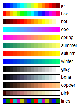
Changing Colormaps

You can change colormaps either interactively:

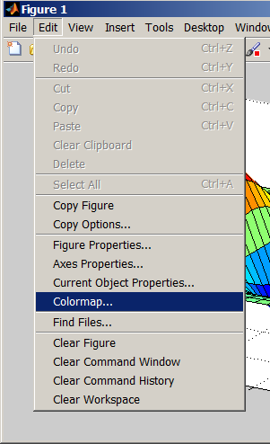
or programmatically:

colormap(cool)

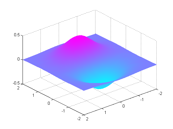
Shading

You can control the shading of surface objects using the shading function.

shading interp

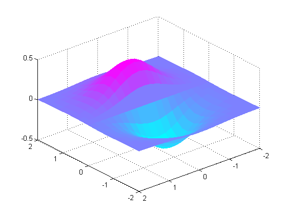
shading flat

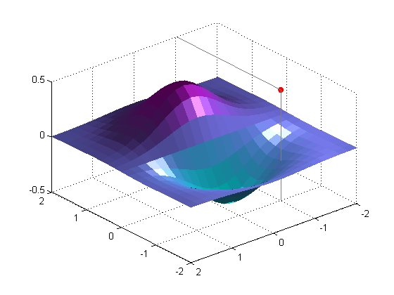
Lighting

You can place a light source at a particular location. Alternatively, you can also use camlight.

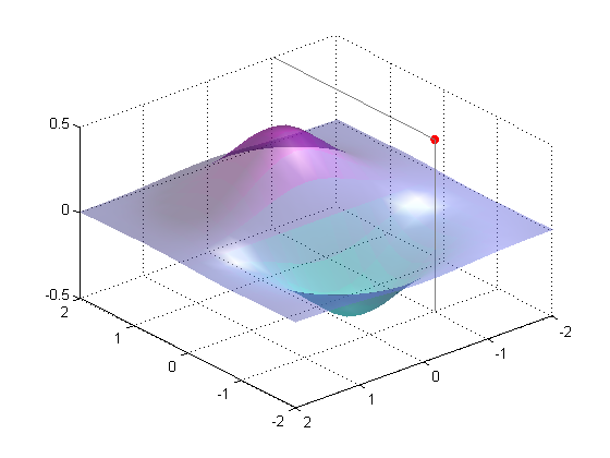
% Light source location
% s = [-2, 0, 0.5];
s = [-1, -1, 0.5];

% Put a point to indicate where the light source is (for reference)
line(s(1), s(2), s(3), 'marker', '.', 'markersize', 20, 'color', 'red')
line([s(1) s(1);2 s(1)], [s(2) s(2);s(2) s(2)], [s(3) s(3);s(3) -0.5], ...
   'color', [.5 .5 .5])

light('Position', s, 'Style', 'local');

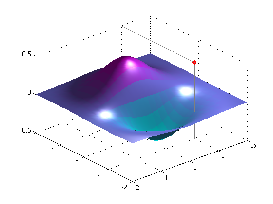
We can select a pre-set lighting algorithm which is good for curved surfaces.

lighting phong

Transparency

You can adjust the transparency with the alpha function.

alpha(0.5)

Table of Contents